
Quantum correlation dynamics in a two-qubit Heisenberg XYZ model with decoherence*
[Yang Guo-Hui† , Zhang Bing-Bing, Li Lei]
, Zhang Bing-Bing, Li Lei]
|
|


†Corresponding author. E-mail: yangguohui_1981_1981@126.com
*Project supported by the Natural Science Foundation for Young Scientists of Shanxi Province, China (Grant No. 2012021003-3) and the Special Funds of the National Natural Science Foundation of China (Grant No. 11247247).
Quantum correlation dynamics in an anisotropic Heisenberg XYZ model under decoherence is investigated by making use of concurrence C and quantum discord (QD). Firstly, we show that both the concurrence and QD exhibit oscillation with time whereas a remarkable difference between them is presented: there is an “entanglement intermittently sudden death” phenomenon in the concurrence but not in the QD, which is valid for all the initial states of this system. Also, the interval time of entanglement sudden death is found to be strongly dependent on the initial states, the inhomogeneous magnetic field b and the anisotropic parameter Δ. Then, it implies that the steady concurrence and QD can be obtained in the long-time limit, which means that the environmental decoherence cannot entirely destroy the quantum correlation, the variation of the uniform magnetic field B and the anisotropic parameter can change the magnitude of the steady concurrence and QD evidently whereas the parameter b cannot. In addition, based on the analysis of the steady concurrence and QD with t →∞, we give the reason why the magnitude of the steady concurrence and QD is so complicated with the change of the parameters B and Δ, whereas the parameter b is independent of the steady concurrence and QD.
As a valuable resource in quantum information and quantum computation, [1, 2] quantum correlation has attracted lots of attention over past years since it provides the possibility of quantum teleportation, [3, 4] quantum dense coding, [5] and quantum cryptographic key distribution, [6] etc. The most fascinating nonlocal correlation feature of quantum mechanics is the quantum entanglement, generally considered as an essential resource for the quantum information processing.[7, 8] Intuitively, we expect that entanglement captures all of the nonclassicality in a correlation. However, recent research reveals that entanglement does not provide all aspects of quantum correlations. For mixed states, nonlocality and entanglement are not identical with quantum correlations. Entanglement is a special kind of quantum correlations, but not the only kind. Recently, many authors have proposed a variety of computable measures to characterize quantum correlations in the composite states: measurement-induced disturbance (MID), [9, 10] quantum discord (QD), [11– 13] geometric discord (GD), [14– 17] measurement-induced nonlocality (MIN), [18] and so on. However, so many useful measurements to characterize quantum correlation lead to a lack of a uniform criterion.
Among these measurements, QD introduced in Ref. [11] is widely used to measure the quantumness of correlation contained in a bipartite quantum state. Some recent results[15, 19] suggest that QD captures the nonlocal correlation more generally than entanglement. Even for some separable states, the entanglement is zero while it can have nonzero QD, which indicates the presence of nonclassical correlation. Due to the good integrability and scalability, the solid state systems have gained great attention.[20– 22] As the natural candidates for the realization of the correlation, spin chains have demonstrated some substantial advantages compared with the other physical systems.[23– 29] They not only have useful applications, but also display rich correlation features.[30– 33] The simplest spin chain, i.e., the Heisenberg chain, has been used to construct a quantum computer and quantum dots.[34– 36] In addition, by suitable coding, the Heisenberg interaction alone can be used for quantum computation.[37– 39] On the other hand, it is well known that decoherence is a vital factor that should not be ignored in quantum information processing. The coupling between any quantum system and its environment is inevitable. Dissipative effects on quantum correlations measured by entanglement in Heisenberg chains have been analyzed in several contexts both in the absence and in the presence of an external magnetic field.[22, 28, 33] Therefore, it is very interesting and necessary to study the quantum correlations in a spin model with decoherence by using other measures. In this paper, several interesting results are obtained based on the behavior of the QD about the effects of external field parameters B, b, and the anisotropic parameter Δ , where many of them are in contrast to the behavior of the entanglement.
In this paper, we will explore the quantum correlation behaviors of a two-qubit anisotropic Heisenberg XYZ chain with environmental decoherence in the presence of a uniform and inhomogeneous magnetic field. In Section 2, we introduce the Hamiltonian of the system and give the master equation which provides the evolution of an open system. In Section 3, we briefly review the definitions about the quantum correlation measures concurrence and QD, respectively. Then the quantum correlation behaviors of our spin system and a detailed comparison between the entanglement and QD are investigated. Conclusions are finally drawn in Section 4.
In this section we first consider the Hamiltonian for an anisotropic N-qubit Heisenberg chain with nearest-neighbor interactions which can be written as
where 

We consider an anisotropic two-qubit Heisenberg XYZ model with external magnetic field, the Hamiltonian H can be written as
where J = (Jx + Jy)/2, γ = (Jx− Jy)/(Jx + Jy), and 
In practical realization, every quantum system is open and unavoidable interaction with the surrounding environment leads to decoherence. The description of the time evolution of an open system is provided by the master equation, which can be written most generally in the Lindblad form with the assumption of weak system– reservoir coupling and Born– Markov approximation.[40, 41] The Lindblad equation for our case thus reads

where { } means anticommutator and γ is the environmental decoherence rate.
For a two-qubit system, mark the four basis states | 00〉 , | 01〉 , | 10〉 , and | 11〉 as 1, 2, 3, and 4, we know that the density matrix contains nonzero elements usually along the main diagonal and anti-diagonal parts, such as the X-state form
for this two-qubits system, prepared in an initial quantum state determined by the X-state initial density matrix ρ (0), after some time the evolution state density matrix ρ (t) remains the X-structure. In order to describe the quantum correlation, we use two measures including concurrence and QD. The concurrence C can be calculated with the help of Wooters’ formula 


On the other hand, one can use the QD to examine quantum correlation dynamics. In classical information theory, the total correlations in a bipartite quantum system are measured by the quantum mutual information

where S(ρ ) = − Tr(ρ log2ρ ) is the Von Neumann entropy, ρ A and ρ B are the reduced density matrices of the subsystems A and B, respectively. The quantum mutual information is usually used as a measure of total correlations that include quantum and classical ones. The classical correlation 𝓒 (ρ AB) is defined as the maximum information about one subsystem, which usually depends on the type of measurement performed on the other subsystem. In this paper, we limit ourselves to projective measurement Π k = | k〉 〈 k| (k = ± ) performed only on the subsystem B, the two orthogonal states | + 〉 and | − 〉 can be represented as a unitary vector on the Bloch sphere | + 〉 = cos θ | 1〉 + eiϕ sin θ | 0〉 and | − 〉 = e− iϕ sin θ | 1〉 − cos θ | 0〉 with 0 ≤ θ ≤ π /2 and 0 ≤ ϕ ≤ 2π . Then the classical correlation can be defined as[9, 11, 13]
the minimum is taken over the complete set of orthogonal projectors Π k, where

is the reduced matrix of subsystem A after obtaining the measurement outcome k, where pk = TrAB[(IA⊗ Π k)ρ AB (IA⊗ Π k)]. Then the difference between the total correlations and the classical correlations can be defined as

which is the so-called quantum discord (QD). Usually, QD is somewhat difficult to calculate and we cannot get the analytical solutions. While for the X-structure density matrix, if we define
with λ i being the eigenvalues of ρ AB, then we can obtain the exact expression of quantum discord as

where
and

In the following, we use the concurrence and QD to study the dynamical characters about the quantum correlation for this two-qubit system prepared in different initial states.
Case 1 If the two-qubit system is prepared initially in the separable initial state | 00〉 . According to the reduced density matrix described by Eq. (3), and substituting Hamiltonian H and ρ (0) into Eq. (3), the explicit form of the nonzero matrix elements are
where ξ 2 = J2Δ 2 + B2, M = γ 2 + 4ξ 2, and E = ξ (2iξ 2 + iγ 2 + γ B)sin(2ξ t) − (2ξ 2B − iξ 2γ + Bγ 2)cos(2ξ t). By knowing the density matrix and the definitions of concurrence and QD, it is convenient for us to obtain the quantum correlation properties.
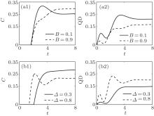
Figure 1 presents the evolution of correlation behaviors with the separable initial state | 00〉 . We see from Fig. 1 that the concurrence and QD oscillate with the increase of time, and the oscillation amplitude of QD behaves like the second peak is roughly larger by a factor than the first peak. Finally, both the concurrence and QD approach a steady value in the long-time limit and adjusting the uniform magnetic field B and the anisotropic parameter Δ will lead the steady concurrence (SC) and steady QD (SQD) to change. One interesting thing is that although C is initially zero for a period of time t, we have nonzero values for QD except the starting point (for the separable initial state, the QD is initially to be the minimum value 0). That is to say the entanglement quantified by C exhibits a “ sudden birth” of entanglement.[45, 46] In contrast to this, QD is always existence. Panels (a1) and (a2) show the concurrence and QD as a function of time with different values of B and the determined values Δ = 0.5. It can be seen that the oscillation of concurrence and QD is weaker with increasing B. On the contrary, panels (b1) and (b2) show the concurrence and QD as a function of time with different values of Δ and the determined values B = 0.5. It can be seen clearly that the oscillation of concurrence and QD get weaker with decreasing Δ .
 | Fig. 1. Time evolution of the quantum correlation calculated by C and QD. Panels (a1) and (a2) for different values of the uniform magnetic field B: B = 0.1 (solid line) and B = 0.9 (dotted line), respectively, with Δ = 0.5; panels (b1) and (b2) for different values of the anisotropic parameter Δ : Δ = 0.3 (solid line) and Δ = 0.8 (dotted line), respectively, with B = 0.5. Other parameters are J = 1 and γ = 1. |
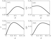
It is worth noting that the remarkable behaviors of the concurrence and QD are presented in Fig. 1, where both the concurrence and QD approach a steady value in the long-time limit and the variation of the uniform magnetic field B and the anisotropic parameter Δ can clearly change the magnitude of the SC and SQD. However, the magnitude of the SC and SQD is very complicated with the change of the parameters B and Δ , there is no uniform conclusion. It can be clearly seen that in Fig. 1 [panel (a1)] the magnitude of the SC increases with the increase of B for the determined value of Δ , while in Fig. 1 [panel (a2)] we observe that the SQD increases with the decrease of B for the determined value of Δ . So one interesting and strange thing is presented: increasing B can improve the SC but decrease the SQD, which means that the effect of the variable B on the SC is entirely opposite to the SQD. In Fig. 1 (panel (b1)), it implies the situation that the magnitude of the SC increases with the decrease of Δ for the determined value of B, however the SQD increase with the increase of Δ for the determined value of B is presented in Fig. 1 (panel (b2)). Also, a strange phenomenon is that increasing Δ can decrease the SC but increase the SQD. This implies that the effect of the variable Δ on the SC is totally opposite to the SQD. In what follows, we will illustrate why this strange phenomenon occurs. In Fig. 2, with the limit case t → ∞ , the SC and SQD behaviors can be obtained in Fig. 2 for the anisotropic parameter Δ = 0.5 [panels (a1) and (a2)], and the uniform magnetic field B = 0.5 [panels (b1) and (b2)]. It is interesting to note that the change of the SC and SQD is nonlinear, it increases first, and undergoes a decreasing procession after it reaches the maximum value of the steady correlation. In Fig. 2 (panel (a1)), the SC increases with B = 0.1 → B = 0.9, whereas an opposite effect for the SQD behaviors is presented (the SQD decreases with B = 0.1 → B = 0.9) in Fig. 2 (panel (a2)). In Fig. 2 (panel (b1)), it shows that the SC decreases with Δ = 0.3 → Δ = 0.8, also an opposite effect is shown in Fig. 2 (panel (b2)) for the SQD behaviors.
 | Fig. 2. With t → ∞ , the steady concurrence and QD behaviors are plotted as a function of B [panels (a1) and (a2)] and Δ [panels (b1) and (b2)]. Other parameters are chosen as J = 1, γ = 1 and panels (a1) and (a2) for Δ = 0.5, panels (b1) and (b2) for B = 0.5. |
Case 2 When the two-qubit system is in the separable initial state | 01〉 . Using Eq. (3), one can obtain the nonzero matrix elements of the evolution density matrix as
where ξ 2 = J2Δ 2 + B2, η 2 = J2 + b2, M = γ 2 + 4ξ 2, and F = (2iξ 2 − Bγ )cos(2ξ t) + ξ (2B + iγ )sin(2ξ t). One can observe that the density matrix contains the inhomogeneous magnetic field b. That is to say, the parameter b can influence the quantum correlation under this initial state. Using the same method, we can obtain the quantum correlation properties.
Figure 3 shows the evolution of correlation behaviors with the separable initial state | 01〉 . It can be seen that both the concurrence and the QD exhibit oscillation with the increase of time. The interesting thing is that if b is smaller (b = 0.05), the concurrence is intermittently death and birth. This means the entanglement sudden death and revival occur after an initial concurrence oscillation and the interval time of entanglement sudden death increases with the increase of time. As b increases (b = 0.2), the entanglement sudden death and revival occur after the second concurrence oscillation and the interval time of sudden death is reduced in comparison with the case of b = 0.05. However there is no sudden death and revival phenomenon in the QD, and the QD decays with time. This means that the quantum correlation based only on the QD is expected to be more robust than that based on the concurrence of this system.
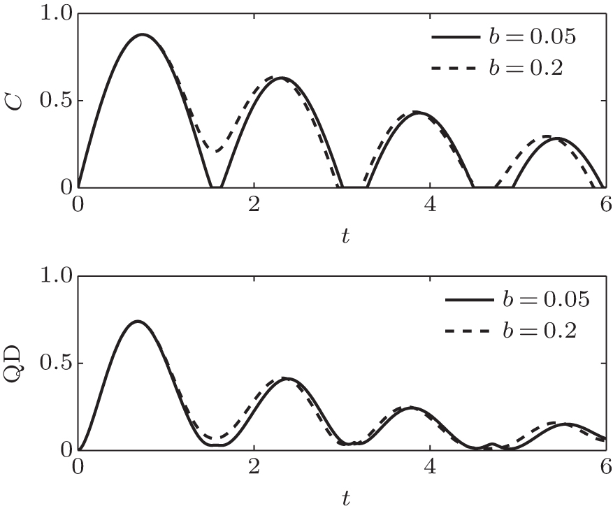 | Fig. 3. Time evolution of the quantum correlation calculated by C and QD with different values of the inhomogeneous magnetic field b: b = 0.05 (solid line) and b = 0.2 (dashed line), respectively. Other parameters are: J = 1, γ = 0.1, Δ = 0.9, and B = 1. |
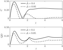
Figure 4 shows the novel features of the concurrence and the QD as a function of time t with the separable initial state | 01〉 . One can see clearly that the “ entanglement sudden death and revival” phenomenon is still quite different between the concurrence and the QD. Specifically, when Δ is larger (Δ = 0.85), the concurrence undergoes twice “ sudden death and revival” phenomenon and finally reaches a steady value in the long-time limit. However, the interval time of the second sudden death is obviously increased in comparison with the first one. As Δ decreases (Δ = 0.4), it only undergoes once “ sudden death and revival” and the interval time of the sudden death is evidently less than the case of Δ = 0.85. In addition, a small Δ leads to extremely strong entanglement and the steady value of entanglement is also increased. It is worth noting that the QD is only in oscillation with the increase of time, there is no sudden death and revival phenomenon. Also, a small Δ leads to extremely strong quantum discord, and the steady value of the QD increases with the decrease of Δ .
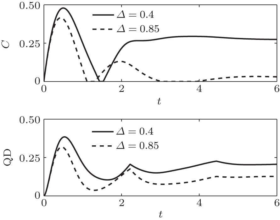 | Fig. 4. Time evolution of the quantum correlation calculated by C and QD with different values of the anisotropy parameter Δ : Δ = 0.4 (solid line) and Δ = 0.85 (dashed line), respectively. For all plots J = 1, γ = 0.8, b = 1, and B = 0.22. |
From the analytic solutions about the density matrix elements under the initial state | 01〉 , we can find that the density matrix contains the inhomogeneous magnetic field b. Though the parameter b can influence some properties of the concurrence and QD, it is independent of the SC and SQD. Now, we give the reason why the variable b cannot make the magnitude of the SC and SQD changes. With the limit case t → ∞ , the explicit form of the non-zero and non-diagonal matrix elements are

it does not contain the parameter b in the matrix elements ρ 14 and 
Case 3 We assume the two qubits are initially in an average entangled state with maximally mixed marginal, which is described by the X-structured density operator
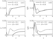
after the time evolution we can get the nonzero matrix elements of the evolution density matrix. To see what happens in the mixed state, we have shown in Fig. 5 the entangled average initial state with C1 = 0.9, C2 = 0.6, and C3 = 0.3. Because of the entangled initial state, it is interesting to find that the concurrence and the QD exist at the beginning of the evolution which is different from the case of the separable pure state. One can clearly see that both the concurrence and the QD oscillate with the increase of time, whereas it also undergoes a sudden death and revival in the concurrence but not in the QD which implies that the concurrence is more fragile than the QD to describe the quantum correlation involved in quantum systems. Also, the steady values of the concurrence and the QD are finally obtained in the long-time limit. However, in panels (a1) and (a2) we see that the steady values of concurrence and QD coincide with each other. It means that the parameter b is independent of the SC and SQD. In panels (b1) and (b2) we observe that the steady values of the concurrence and QD increase with the increase of Δ . In addition, one interesting thing is that the interval time of the entanglement sudden death is enhanced with the decrease of b for the determined value Δ (it is the same with the initial state | 01〉 in Fig. 3). With the determined value of b, the interval time of the entanglement sudden death increases with the decrease of Δ , and it is obvious that the effect of the variable Δ on the sudden death interval time is entirely opposite to the initial state | 01〉 (the interval time of the sudden death increases with the increase of parameter Δ ) in Fig. 4. That is to say, the interval time of entanglement sudden death is found to be strongly dependent on the initial states and the parameters b and Δ .
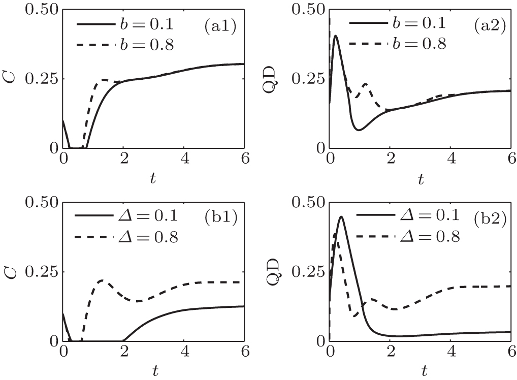 | Fig. 5. Time evolution of the quantum correlation calculated by C and QD. Panels (a1) and (a2) for different values of the anisotropic parameter b: b = 0.1 (solid line) and b = 0.8 (dotted line), respectively, with Δ = 0.5; panels (b1) and (b2) show different values of the anisotropic parameter Δ : Δ = 0.1 (solid line) and Δ = 0.8 (dotted line), respectively, with b = 0.5. Other parameters are: C1 = 0.9, C2 = 0.6, C3 = 0.3, J = 1, γ = 1, and B = 0.5. |
In conclusion, we illustrate the quantum correlation properties about an anisotropic two-qubit Heisenberg XYZ system under decoherence. The results show that the concurrence and QD can behave very differently with time for different initial states. We show that both the concurrence and the QD oscillate with time, while a clear difference between the behaviors of the concurrence and the QD is that there is a sudden death and revival phenomenon in the former but not in the latter, and the interval time of entanglement sudden death is found to be strongly dependent on the initial states, the parameters b and Δ . This implies that the QD is more robust than the concurrence to describe the quantum correlation involved in quantum systems. We also explore the different effects of the coupling parameters on the concurrence and QD behaviors. The results show that the steady concurrence and QD can be obtained in the long-time limit, which indicates that the environmental decoherence cannot entirely destroy the quantum correlation, and different values of the uniform magnetic field B and the anisotropic parameter Δ can change the magnitude of the SC and SQD, while the parameter of the inhomogeneous magnetic field b cannot. In addition, based on the analysis of the SC and SQD with the limit case t → ∞ , we give the reason why the magnitude of the SC and SQD is so complicated with the change of the parameters B and Δ , whereas the parameter b is independent of the SC and SQD.
| 1 |
|
| 2 |
|
| 3 |
|
| 4 |
|
| 5 |
|
| 6 |
|
| 7 |
|
| 8 |
|
| 9 |
|
| 10 |
|
| 11 |
|
| 12 |
|
| 13 |
|
| 14 |
|
| 15 |
|
| 16 |
|
| 17 |
|
| 18 |
|
| 19 |
|
| 20 |
|
| 21 |
|
| 22 |
|
| 23 |
|
| 24 |
|
| 25 |
|
| 26 |
|
| 27 |
|
| 28 |
|
| 29 |
|
| 30 |
|
| 31 |
|
| 32 |
|
| 33 |
|
| 34 |
|
| 35 |
|
| 36 |
|
| 37 |
|
| 38 |
|
| 39 |
|
| 40 |
|
| 41 |
|
| 42 |
|
| 43 |
|
| 44 |
|
| 45 |
|
| 46 |
|