Degree distribution and robustness of cooperative communication network with scale-free model*
[Wang Jian-Rong, Wang Jian-Ping† , He Zhen, Xu Hai-Tao]
, He Zhen, Xu Hai-Tao]
 |


†Corresponding author. E-mail: jpwang@ustb.edu.cn
*Project supported by the Natural Science Foundation of Beijing (Grant No. 4152035) and the National Natural Science Foundation of China (Grant No. 61272507).
With the requirements of users enhanced for wireless communication, the cooperative communication will become a development trend in future. In this paper, a model based on complex networks with both preferential attachment is researched to solve an actual network CCN (Cooperative Communication Network). Firstly, the evolution of CCN is given by four steps with different probabilities. At the same time, the rate equations of nodes degree are presented to analyze the evolution of CCN. Secondly, the degree distribution is analyzed by calculating the rate equation and numerical simulation. Finally, the robustness of CCN is studied by numerical simulation with random attack and intentional attack to analyze the effects of degree distribution and average path length. The results of this paper are more significant for building CCN to programme the resource of communication.
With the development of wireless communication technology, not only the requirements of data rate and quality of service are constantly improved for wireless transmission, but also the indicators of the communication system are required higher and higher. Compared with a cable channel, it is more difficult and complex for a wireless channel environment to propagate the radio wave. There are a large number of direct waves, reflected waves, and diffracted waves, which produce a multipath effect, and lead to receiving an unstable signal of wireless communication.
Because the wireless spectrum resources are very scarce, the important problems of wireless communication for achieving a balance between validity and reliability are researched to resist multipath fading and to greatly improve the spectrum utilization. Therefore, the MIMO (Multi-Input Multi-Output) antenna system has been used for increasing the system bandwidth, antenna transmission power, and the capacity of the communication system.[1– 3] The terminal equipment is restricted by volume, hardware complexity, and power consumption, confining the use of the MIMO antenna system. Hence, cooperative communication has been presented as a new space diversity technology.[4– 7] The basic idea of cooperative communication is: In a multi-user communication environment, a virtual antenna array is formed by the cooperative nodes of single antenna terminals. With the continuous requirements for wireless communication, cooperative communication will become a development trend in the future.[8] In recent years, a large number of achievements have been created for cooperative communication such as coding theory, [9, 10] power allocation, [11, 12] relay selection, [13, 14] information security, [15– 17] and so on.
Complex networks play important roles in researching the functional properties of complex systems, and focus on the topology structure of a complex system for interaction among the individuals. Complex networks have been permeated into many academic disciplines, such as sociology, biology, epidemiology, ecology, communication system, and many other fields. Watts and Strogatz presented the small-world model (WS Model), [18] describing the differences and conversions between a completely regular network and a completely random network. Barabasi and Albert presented the scale-free model (BA Model), [19] containing both growth and preferential attachment widely existing in real networks. The properties of the evolving network have been studied by some extended models of the scale-free one for a more realistic description of the local processes, incorporating the addition of new nodes, new links, and the rewiring of links.[20– 22] They analyzed the changing organizational communications structure in order to investigate the patterns associated with the final stages of an organizational crisis.[23]
As a kind of real network, cooperative communication networks (CCN) have been studied by the method of game theory and optimization theory. However, it is difficult to solve the problem of large-scale networks. On the contrary, complex networks are the best theoretical basis to solve these problems usually. It is a shame that there is little research in this field. The growth characteristics of CCN are followed by the BA model. Hence, the scale-free model of complex networks will be considered to apply to CCN in this paper.
In CCN, the nodes with good condition or better performances such as lower BER (Bit Error Rate) are more attractive to other nodes. As new nodes or links are added to the network, there is a tendency for an already heavily linked node (e.g. Base Station) to acquire more attachments. In terms of the quantity, it should contain the component preferential attachment. In particular, we assume the probability expression of nodes attachments in the networks as follows:

where, k(i, t) represents the degree of the node i at time t. pi is the fitness probability of degree for each node, here 0 < pi ≤ 1 and all pi = p in this paper.
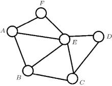
Network Initialization: Starting with m0 nodes existing in the network. The degree of each node is one at least to make sure that there are no isolated nodes in the network. There is at most one relay node for each group of cooperative communication. The steps occur by the probabilities for adding node, adding link, deleting node, and deleting link in per unit time, if six nodes are contained in the network and connected as Fig. 1 at time t – 1.
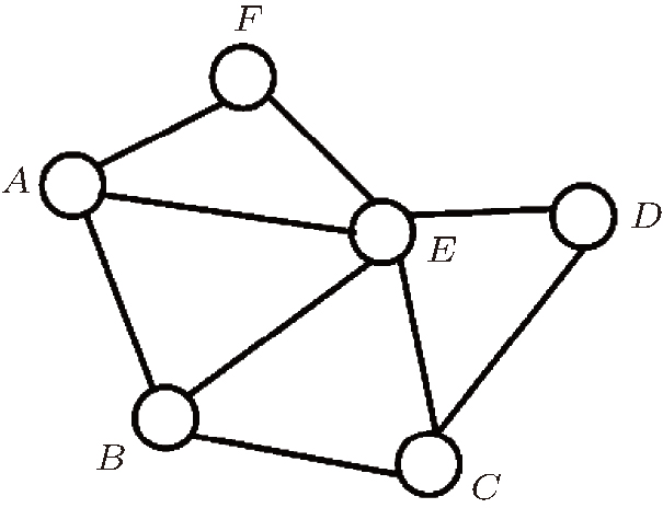 | Fig. 1. The network at time t – 1. |
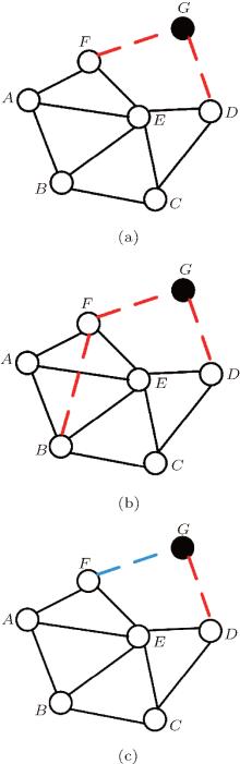
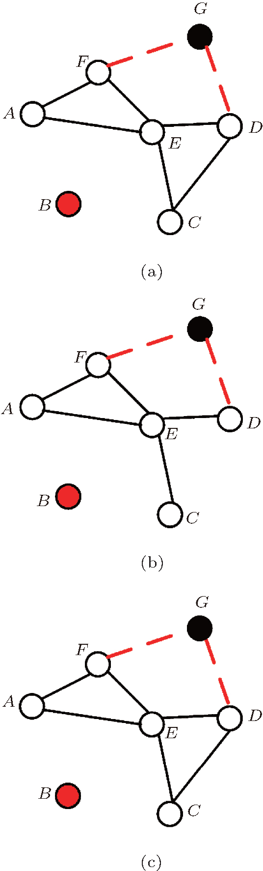
Step 1 With probability p1, a new node will join in the network and start communication with m1 nodes already existing at time t. For instance, in Fig. 2(a), a new node G can join the network and start communication with the node F and node D. The node G and node F (or D) are non-cooperative communication with probability α . The link GF is the edge of cooperative communication group AFG or EFG with probability β . The node G is a relay node for a cooperative communication group FGD with probability γ . In the evolution of CCN, each pair of nodes will want to communicate, a new node must be added or a new connection be established. Then only three communication situations of the pair of nodes are non-cooperative communication (direct communication), using one link of the third node for cooperative communication and using two links of the third node for cooperative communication. So we let α + β + γ = 1. According to the principle and continuum theory, assuming the i-th node to be in the network at time t, the change rate of degree k(i, t) can be written as:
where, N(t) is the total number of nodes in CCN at time t. 〈 k〉 is average degree of CCN which is expressed by ∑ jpk(j, t) at time t. 
 | Fig. 2. Adding nodes and links into CNN. |
Step 2 With probability p2, a new communication link is generated between two nodes already existing at time t in the network. For instance, in Fig. 2(b), the new link BF is non-cooperative communication with probability α . The new link BF is the edge of the cooperative communication group except BFG such as AFB, EFB, or CBF with probability β . The new link BF is the edge of cooperative communication group BFG with probability γ . In Fig. 2(c), the new link FG is non-cooperative communication with probability α . The new link FG is the edge of cooperative communication group AFG or EFG with probability β . The new link FG (G is a relay node) is the edge of cooperative communication group BFG with probability γ . Note that α + β + γ = 1. According to the principle and continuum theory, assuming the i-th node to be in the network at time t, the change rate of degree k(i, t) can be written as
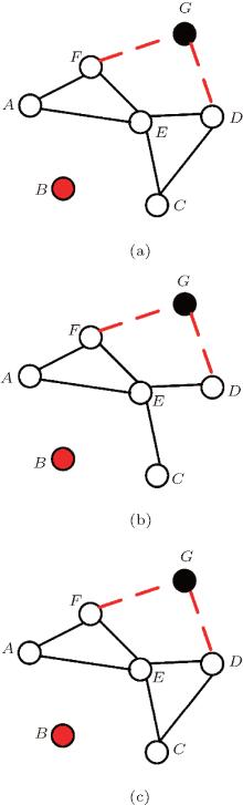
Step 3 With probability p3, an existing node at time t in the network will be deleted and simultaneously cancel its m2 communication links. For instance, in Fig. 3(a), a new node B is deleted from the network, and thus broke off all the communications with others. The deleted node B and node A (or E, C) is non-cooperative communication with probability α . The deleted link BA (or BE, BC) is the edge of cooperative communication group BAF (or BEF, BCD) with probability β . The deleted node B is a relay node for a cooperative communication group ABE, ABC, or EBC with probability γ . Note that α + β + γ = 1. According to the principle and continuum theory, assuming the i-th node to be in the network at time t, the change rate of degree k(i, t) can be written as
Step 4 With probability p4, an existing communication link is deleted at time t in the network. For instance, in Fig. 3(b), the deleted link CD is non-cooperative communication with probability α . The deleted link CD is the edge of cooperative communication group except BCD such as ECD, or GCD with probability β . The deleted link CD is the edge of cooperative communication group BCD with probability γ . In Fig. 3(c), the deleted link BC is non-cooperative communication with probability α . The deleted link BC is the edge of cooperative communication group BCD (or BCE) with probability β . The deleted link BC (C is a relay node) is the edge of cooperative communication group ABC with probability γ . Note that α + β + γ = 1. According to the principle and continuum theory, assuming the i-th node to be in the network at time t, the change rate of degree k(i, t) can be written as

 | Fig. 3. Deleting nodes and links from CNN. |
In evolution of CCN, there are only four steps with different probabilities at time t. But these steps are independent, and only one event occurs in a unit time. The process of evolution CCN will be repeated according to the above four steps until the network reaches to a certain scale and note that p1 + p2 + p3 + p4 = 1.
In this section, to derive the scaling law for P(k), it is necessary to obtain the temporal evolution of the connectivity for a given node. The equations of the degree growth rate for CCN shown above are presented, respectively. By adding the rate equations of the above four steps such as Eqs. (1), (2), (3), and (4), we obtain the following dynamical equation

where,
N(t) = (1 – p3)t is the total number of nodes in the network at time t. S(i, t) is the probability that node i is not deleted and still stays in the network at time t. Then, 
Using independence of the events corresponding to random deletions of nodes at each time step, it is easy to verify that

Hence, the continuous version of the dynamics of S(i, t) can be stated as follows:

Since, S(t, t) = 1, k(t, t) = m1, we get

It is easy to solve the K(t) and 〈 k〉

Inserting Eq. (7) back into Eq. (5), we get

where,

Together with the initial conditions S(t, t) = 1 and k(t, t) = m1, we obtain the solution to Eq. (8) written as follows:
for t → ∞ and 0 < p ≤ 1.
Now the degree distribution of CCN is calculated as follows:
This is a power-law distribution with the exponent λ = − 1 + 1/(E(p3 − 1)). This equation for obtaining the power-law exponent from Eq. (9) for a general case will be used later.
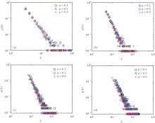
In order to check the analytical results obtained in this paper, we have performed extensive numerical simulations of the degree and degree distribution. The numerical simulations of degree distribution with N = 1000 are shown in Fig. 4 and other values of parameters are shown as p = 0.1, 0.5, 0.9, p1 = 0.4, p2 = 0.26, p3 = 0.08, p4 = 0.26, α = 0.25, β = 0.7, γ = 0.05, m1 = 3, 5, 7, 9, m2 = 3. With the growth nodes in CNN, we can see that the degrees of some nodes are increased from the degree distribution which follows the forms of power-law for p = 0.1, 0.5, 0.9.
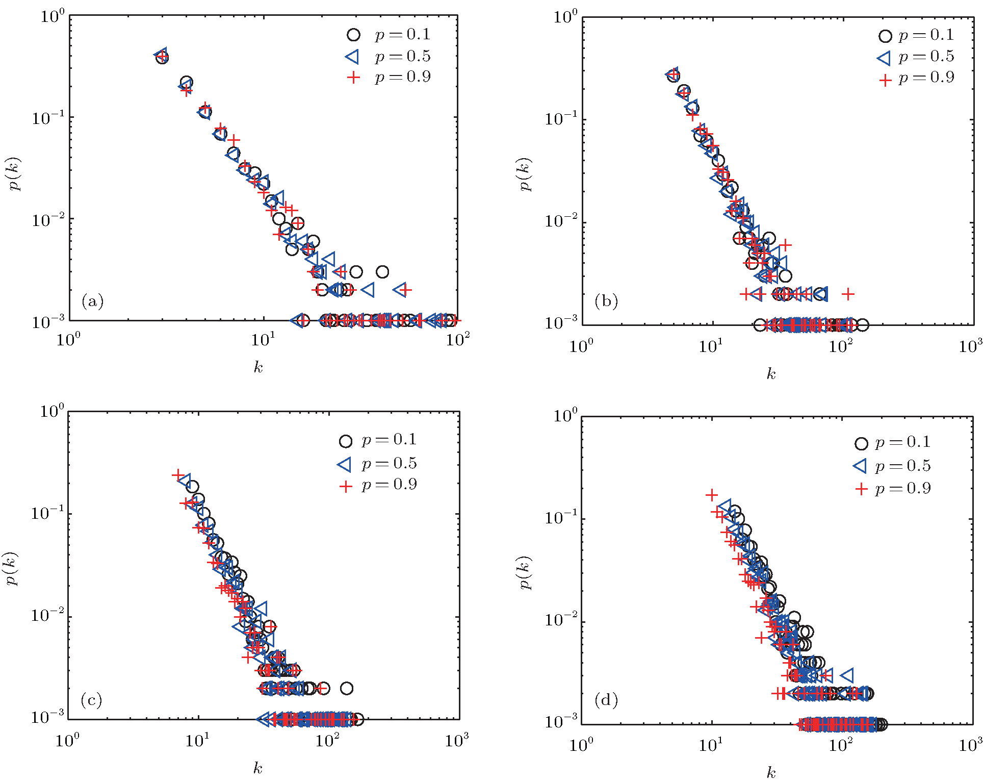 | Fig. 4. Degree distribution with different m1 = 3 (a), 5 (b), 7 (c), and 9 (d). |
The robustness is an important indicator for network topology to measure the performance of self-organization. Normalized average edge betweenness of a network as a metric of network vulnerability was considered.[24] A fluid-flow model for TCP (Transmission Control Protocol) congestion avoidance combined with different AQM (Active Queue Management) schemes is analyzed.[25] The research had revealed that real complex networks are inherently vulnerable to the loss of high centrality nodes.[26] In this section, we will investigate robustness of CCN with topological structure which is emerged by a mixture of both power-law and exponential degree distributions. Average path length L and average degree 〈 k〉 are two of the main factors to influence the robustness of network, and are defined as follows:

where, di j is devoted by the number of links for the shortest path between node i and node j.
Here, we consider the effect of random nodes attack and intentional nodes attack to analyze the properties of CCN. Random nodes attack: Randomly choosing one of the nodes in CCN and removing all its links. Intentional nodes attack: Finding a node with the maximum degree in CCN and removing all its links. If several nodes happen to the same highest degree of connection, we will randomly choose one of them.
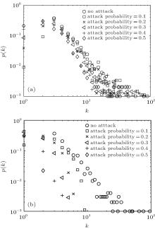
In Fig. 5, the degree distribution of CCN is shown for two attacks with different attack probabilities, which are denoted by the presence of attacked nodes and total nodes. The parameters are chosen as p = 0.5, p1 = 0.4, p2 = 0.26, p3 = 0.08, p4 = 0.26, α = 0.25, β = 0.7, γ = 0.05, m1 = 3, m2 = 3, N = 1000, attack probability= 0, 0.1, 0.2, 0.3, 0.4, 0.5. From Fig. 5, with increasing the attack probability, it is easy to see that the tails of degree distribution are shorter and shorter by two attack methods. But it is more observable for the effect of degree distribution by intentional attack than random attack. The reasons for this situation are caused by most of the nodes in CCN with smaller degrees.
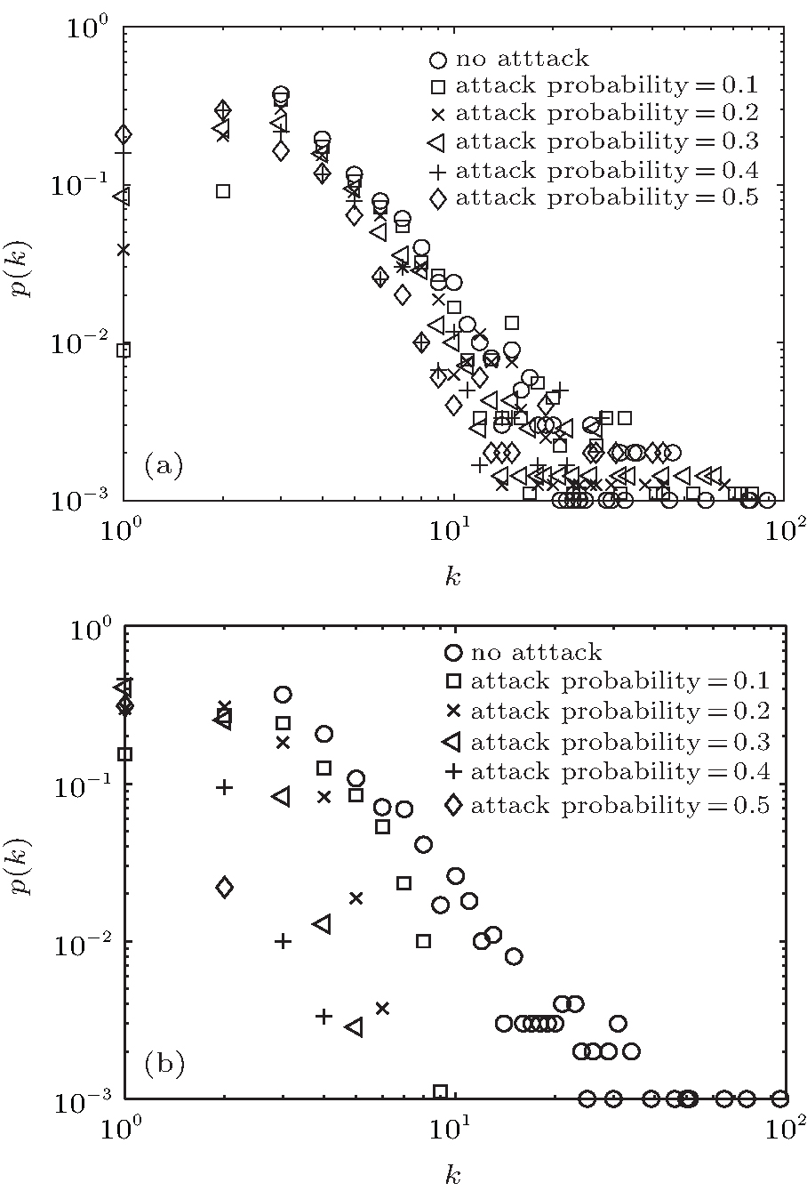 | Fig. 5. The effect of degree distribution with different attacks: (a) random attack degree distribution and (b) intentional attack degree distribution. |
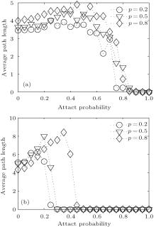
In Fig. 6, the average path length of CCN is shown for two attacks with different attack probabilities. The parameters are chosen as p = 0, 0.5, p1 = 0.4, p2 = 0.26, p3 = 0.08, p4 = 0.26, α = 0.25, β = 0.7, γ = 0.05, m1 = 3, m2 = 3, N = 1000, attack probability = 0, 0.05, 0.1, … , 0.95, 1. From Fig. 6, with increasing the attack probability, it is easy to see that the average path length will grow longer and longer. When the attack probability increased to a certain extent, there are more separated small clusters, which will lead to the average path length becoming smaller and smaller and finally tending to 0. As p increased, it is more effective for CCN to resist the intentional attack than the random attack. However, the average path length is influenced by the intentional attack more seriously than by the random attack.
 | Fig. 6. The effect of average path length with different attacks: (a) average path length of random attack and (b) average path length of intentional attack. |
In this paper, a model of complex networks with preferential attachment has been researched and applied to CCN. The evolution of CCN has been given by four steps with different probabilities such as adding node, adding link, deleting node, and deleting link. At the same time, the rate equations of nodes degree have been presented to analyze the evolution of CCN. Then, the degree distribution has been analyzed by calculating the rate equation and numerical simulation. With the growth nodes in CNN, the degrees of some nodes have been increased by analyzing the degree distribution with the forms of power-law. Finally, the robustness of CCN has been studied by numerical simulation with random attack and intentional attack to analyze the effects of degree distribution and average path length. Compared with the intentional attack, CCN had better resistance for the random attack. But with growing p or 〈 k〉 , the resistance of CCN is improved by the intentional attack.
In the future studies, we will investigate a kind of adaptive model for evolving CCN, which can thoroughly resolve the congestion problems of communication nodes. In addition, it is interesting to analyze the optimal performance of CCN with a combined attack of the random attack and the intentional attack.
The authors are very grateful to the reviewers and editors for their insightful comments and suggestions.
| 1 |
|
| 2 |
|
| 3 |
|
| 4 |
|
| 5 |
|
| 6 |
|
| 7 |
|
| 8 |
|
| 9 |
|
| 10 |
|
| 11 |
|
| 12 |
|
| 13 |
|
| 14 |
|
| 15 |
|
| 16 |
|
| 17 |
|
| 18 |
|
| 19 |
|
| 20 |
|
| 21 |
|
| 22 |
|
| 23 |
|
| 24 |
|
| 25 |
|
| 26 |
|