The wave– flow interaction is an important subject of atmospheric dynamics. The flow is referred to as the basic-state flow and the wave is a deviation from the basic-state flow. Their interaction includes two aspects: the feedback to the basic-state flow from the wave, which is described by the E– P flux theory, ^{[1– 4]} and the forcing to the wave by the basic-state flow, which is presented by the wave-activity relation.^{[5– 10]} Because the basic-state flow and the wave vary with different temporal scales, the two aspects can be investigated individually. The wave-activity density, which is quadratic (or of higher order) in the disturbance fields, can be a conserved quantity at the small-amplitude limit.^{[11, 12]} Generally, the wave-activity density satisfies the following wave-activity relation in flux form:

where A and F are the wave-activity density and the wave-activity flux, respectively, and S is the source or sink. In the absence of diabatic heating and turbulent dissipation, S tends to be zero, and the above equation becomes conserved. Then, the tendency of the wave-activity density is controlled by the convergence or divergence of the wave-activity flux. Many studies have shown that the wave-activity relation provides a theory that underlies the interaction between the basic state flow and the wave.^{[13– 15]}

Popular methods to construct such a relation include the momentum-Casimir and the energy-Casimir methods, which were used by Arnol’ d and others to prove stability theorems for some conservation flows.^[16] McIntyre and Shepherd, ^[17] Haynes, ^[12] and Scinocca et al.^[11] extended these methods to investigate the wave-activity relations for small-amplitude and finite-amplitude disturbances to parallel and nonparallel flows. Ran and Gao employed the momentum-Casimir method to construct the pseudomomentum wave-activity relation for dry air in the nonhydrostatic dynamic framework.^[18] The wave– flow interaction was theoretically examined by Ran and Boyd, and its two aspects were linked via the basic-state diabatic heating.^[19]

Previous investigations of the wave– flow interaction have mostly been confined to large-scale systems. However, the severe precipitations leading to flood disasters are often associated with the meso-scale systems, and for some time have also attracted much attention.^{[20– 25]} Recently, wave-activity relations were also applied to heavy-rainfall event diagnosis. Ran et al. analyzed the dynamic processes responsible for precipitation during the landfall of typhoon Wipha in terms of the wave-activity density.^[26] Since the wave-activity density is capable of describing the typical vertical structure of dynamic and thermodynamic fields, it presents anomalies in the middle and lower troposphere over the strong precipitation area.^[27] Chu et al. developed the potential shear wave-activity relation and investigated the meso-scale features in typhoon Morakot’ s (2009) precipitation.^[28]

In previous studies of the wave-activity relation, moisture was not explicitly taken into account. The real atmosphere, however, is not truly dry. It contains moisture and is often saturated when heavy rainfall occurs. Thus, it is quite necessary to extend the previous study of Ran and Gao, ^[18] and derive a new wave-activity relation involving moisture to diagnose the energetics of meso-scale systems which have interactions with the large-scale basic flow in real moist atmosphere. To realize this, the present paper employs the energy-Casimir method to derive a three-dimensional non-hydrostatic virtual pseudoenergy wave-activity relation in the presence of various hydrometeors and related moist processes. The governing equations are presented in Section 2. The virtual pseudoenergy wave-activity relation for moist atmosphere is derived in Section 3. The results are summarized in Section 4.

Consider a diabatic, viscid, compressible, and moist atmosphere. The governing equations on β -plane in Cartesian coordinates (x, y, z, t) are given by

where is the virtual temperature; θ _v is the virtual potential temperature; T is the temperature; λ = 1.608 is a constant; v = (u, v, w) is the three-dimensional velocity; p is the pressure; ρ is the total density of moist atmosphere, which is the sum of dry-air density ρ _d, water-vapor density ρ _v, cloud-water density ρ _c, rain-water density ρ _r, ice density ρ _i, snow density ρ _s, and graupel density ρ _g; Q_v is the water-vapor mixing ratio; Q_l is the mixing ratio sum of cloud water Q_c, rain water Q_r, ice Q_i, snow Q_s, and graupel Q_g; w_r, w_s, and w_h are the terminal velocities of rain water, snow, and graupel, respectively; θ = T(1000/p)^R/c_p is the potential temperature; R is the dry-air constant; c_p is the specific heat at constant pressure; g is the gravitational acceleration; f₀ is the Coriolis parameter; β is the Rossby parameter; and, k is the unit vector in the vertical direction. In addition, S_θ is the diabatic heating; S_Qv is the source or sink for Q_v; and, D_u, D_v, D_w, D_θ , D_Qv, and D_Ql denote the dissipations of momentum, potential temperature, and water substances, respectively. As an equation system involving water substances, equations  (2)– (8) have been extensively employed in numerical models such as the weather research and forecasting model (WRF), ^[29] the advanced region prediction system (ARPS), ^[30] and the cloud-resolving model.^[31]

By using Eqs.  (3), (5), and (6), one obtains the continuity equation of total mass

where

and

is the mass forcing composed by fallouts of Q_r, Q_i, and Q_g at their respective terminal speeds and dissipations of water substances. Qiu et al. examined the significance of mass forcing and found that the mass forcing is important in the numerical simulations of heavy rainfall.^[32] The mass forcing resulting from heavy rainfall may cause the anomaly of moist potential vorticity.^[33] These studies suggest that the effect of mass forcing on heavy precipitation is not negligible.

The total energy equation is given by

where E = (u² + v² + w²)/2 + gz + c_vT_v is the virtual energy density, which is the sum of kinetic energy, potential energy, and virtual internal energy c_vT_v, and

is the source or sink for the energy density. The right-hand side terms in Eq.  (11) stand for the contributions of thermal source and dissipation, moisture source and dissipation, momentum dissipations, and mass forcing, respectively. For adiabatic, inviscid, and dry atmosphere, equation (10) is a conservation equation of energy.

By taking moisture into account, the virtual potential vorticity (VPV) is expressed as

where ω = (∂ w/∂ y − ∂ v/∂ z, ∂ u/∂ z − ∂ w/∂ x, ∂ v/∂ x − ∂ u/∂ y + f₀ + β y) is the absolute vorticity. The tendency equation of VPV is written as

where

is the source or sink of VPV, and

is the source or sink of θ _v, which contains thermal source and dissipation, moisture source and dissipation, and mass forcing. In the absence of a source or sink for virtual potential temperature, dissipations and mass forcing, VPV satisfies a local conservation equation.

Following Haynes, ^[12] we exploit the Casimir function C = C(q, θ _v), a single-valued algebraic function of q and θ _v. In the conservative case, C is constant following the fluid motion. It satisfies

After adding the energy equation  (10) to the Casimir equation  (16) and using the total continuity equation  (9), one can obtain

where

is the source or sink.

Based on Eq.  (17), we now use the energy-Casimir method^[12] to construct the virtual pseudoenergy wave-activity relation for a moist atmosphere. The Casimir function C is chosen to make the difference between ρ (E + C) and its basic state equal to the divergence of a flux plus a second-order wave quantity and a basic-state quantity. As pointed out by Scinocca and Shepherd, ^[11] the energy-Casimir method requires the basic states to be stationary.

Before further derivation, it is necessary to discuss the basic states. Let (u₀, v₀, p₀, T₀, ρ ₀, θ ₀, θ _v0, q_v0, q₀) denote the basic states of (u, v, p, T, ρ , θ , θ _v, q_v, q), and take the basic-state values of w and q_l to be zero. These basic-state variables are functions of three-dimensional space variables (x, y, z) and are independent of time. As a steady solution to the governing equations, the basic states satisfy

where v₀ = (u₀, v₀, 0). The thermal– wind relation can be derived as

Let (u_e, v_e, w_e, p_e, T_e, ρ _e, θ _e, θ _ve, q_ve, q_le, q_e) denote the disturbances to the basic states, which is a function of x, y, z, and t. After neglecting the terms that are quadric and higher-order in disturbance amplitude, and reserving all of the source or sink and dissipations, one obtains the linearized disturbance equations

in which v_e = u_ei + v_ej + w_ek is the three-dimensional perturbation velocity and the Taylor series expansion has been used.

Under the assumption that | p_e/p₀| < 1, | ρ _e/ρ ₀| < 1, | T_e/T₀| < 1, | θ _ve/θ _v0| < 1, and | Q_ve/Q_v0| < 1, one can linearize θ _v and p by subtracting the basic-state equations  (24) and (26) from the state equation (15) and θ _v, respectively. Consider the leading-order contributions

Eliminating p_e in Eqs.  (33) and (34) yields

As a disturbance to the basic-state VPV, q₀ = ω ₀ · ∇ θ _v0/ρ ₀ (ω ₀ = (− ∂ v₀/∂ z, ∂ u₀/∂ z, ∂ v₀/∂ x − ∂ u₀/∂ y + f₀ + β _y)) is the basic-state absolute vorticity. The q_e is given by

where ω _e = ∇ × v_e is the perturbation relative vorticity. By performing a Taylor series expansion of C at q = q₀ and θ _v = θ _v0, and considering the quadric contributions to C, one has

where C₀ = C(q₀, θ _v0) is the basic-state Casimir function.

We perform a Taylor series expansion of the quantity ρ (E + C(q, θ _v)) after the substitution of u = u₀ + u_e, v = v₀ + v_e, w = w_e, T_v = T_v0 + T_ve, q = q₀ + q_e, θ _v = θ _v0 + θ _ve. By eliminating T_e and q_e in the leading-order terms of the expansion with Eqs.  (35) and (36), and neglecting the cubic and higher-order contributions, we may rewrite the quantity as

where

is second-order in disturbance amplitude and is called the virtual pseudoenergy wave-activity density for a moist atmosphere. The basic-state Casimir function C₀ = C(q₀, θ _v0) is the evaluation of C at q = q₀ and θ _v = θ _v0.

Following Haynes and Ran et al., we can choose C₀ to make the second, the fourth, and the fifth terms on the right-hand side of Eq.  (38) vanish. This requires C₀ to satisfy

The constraints (41) and (42) are trivially satisfied when equation  (40) is satisfied by the chain rule. It is easy to prove that equations (40)– (42) hold identically by taking the spacial partial derivatives of Eq.  (40) with respect to y and z to eliminate ∂ C₀/∂ q₀ in Eqs.  (41) and (42). The inherent consistency means that a solution of C₀ to Eq.  (40) also satisfies Eqs.  (41) and (42).

By using Eqs.  (40)– (42), equation  (38) becomes

Employing Eqs.  (40)– (42) again, equation  (43) is further simplified as

After substituting Eq.  (43) into the first term on the left-hand side of Eq.  (17) and Eq.  (44) into the second term on the left-hand side of Eq.  (17), one may obtain

Since the disturbance is assumed to be small-amplitude, the terms cubic in disturbance amplitude are neglected. Thus, the above equation may be rewritten as

where

is interpreted as the virtual pseudoenergy wave-activity flux, which is quadric in disturbance amplitude,

is the leading-order perturbation flux, and

is the basic-state flux.

It can be demonstrated that (see in Appendix A)

and

Thus, the virtual pseudoenergy wave-activity relation may be obtained from Eq.  (46) as

where

is the source or sink caused by diabatic heating, dissipation, and mass forcing. Equation (52) shows that the virtual pseudoenergy wave-activity relation takes a local non-conservative form. Its non-conservation results from the diabatic heating, source, or sink and dissipation of q_v, mass forcing, and momentum dissipation. For dry air, the water substance and mass forcing vanish so that θ _v reduces to θ and equation (52) becomes the dry-air pseudoenergy wave-activity relation. If the forcing effects are not taken into account, then the dry-air pseudoenergy wave-activity is subjected to a local conservation form. If the moist atmosphere is unsaturated, which means there are not cloud hydrometeors and phase change of water substance, then the contribution of cloud hydrometeors to A in Eq.  (39) vanishes. Equation (52) is important at two points. One is that the relation is built in the non-hydrostatic and ageostrophic dynamic framework. This indicates that the relation is capable of diagnosing meso-scale systems. The other is that it involves water vapor and is applicable to the saturated and unsaturated moist atmosphere, which is not contained in other wave-activity theories.

In the practical application of Eq.  (52), how to calculate C is crucial, which may be overcome through two ways. One is that C₀ is firstly calculated by numerically solving the integrated expression of C₀ in Eq.  (40) with grid data, and then the known C₀ is interpolated at q and θ _v to evaluate C = C(q, θ _v), just as Durran did. The other is to specify the expression of C in advance, such as in which γ is an arbitrary constant, q_s and θ _vs are the constant reference values of q and θ _v, respectively. Then, the specified expression of C is brought into Eq.  (40), and is then combined with the basic-sated equations  (19)– (25) to evaluate the basic-state quantities with the given grid data by a numerical iteration method.

The wave-activity density represents some kind of wave energy and is an important variable in the wave– flow interaction theory. In order to validate the virtual pseudoenergy wave-activity density in relation (52), it is diagnosed in the following case study.

This section focuses on two cases of heavy precipitation. One is a strong convection case which took place in the west of China on July 8, 2009, resulting in heavy rainfall. In this process, the precipitating system moved eastwards slowly in the belt of 36°   N– 39°   N. The other precipitation case occurred at 1200 UTC August 18, 2009– 0600 UTC August 19, 2009. In this case, the precipitation started in the north of Shanxi province and the middle of Inner Mongolia at 1200 UTC August 18, 2009 and then propagated northeastwards quickly. In these two cases, we examine the capabilities of virtual pseudoenergy wave-activity density A in diagnosing heavy rainfall, its physical meaning is also discussed.

3.2. Result

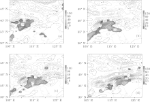
To analyze the integral characteristics of A in the troposphere, we calculate the vertical mean of A. Its horizontal distribution characteristics in the two events are examined. Figure  1 presents the horizontal distributions of A at 0000 UTC, 0600 UTC, 1200 UTC, and 1800 UTC July 8, 2009. It can be seen that in the whole heavy-rainfall process, the positive-value regions of A correspond well with the observed 6-h precipitation regions. The anomaly of A changes with the evolutions of the precipitating system or heavy-rainfall areas. What should be noticed is that A has a high positive value in the non-precipitation region because of its anomalous value in the upper troposphere. The negative-value A region is close to the positive-value A region. Thus, they form a fluctuating pattern. The precipitation is almost located in the positive amplitude region. Further analysis shows that the term is the chief composition of A (the figures are omitted due to space limitations). Since the term ∂ C₀/∂ q₀ is invariant with time, the term A_chief mainly represents the temporal variation of the second-order potential vorticity (ω _e · ∇ θ _ve). The analysis also reveals that the term ω _e · ∇ θ _ve is mainly dominated by the barotropic component of perturbation PV (namely, ). The perturbation θ _ve increases with height in the mid-lower troposphere over the precipitation region, meaning . Moreover, there exists a strong perturbation of the cyclonic vorticity (namely, ) (the figures are omitted due to space limitations). The two factors are important dynamic and thermodynamic characteristics of precipitation. They present high values over the precipitation region, which further results in the positive anomalies of ω _e · ∇ θ _ve, A_chief, and A. The anti-cyclonic vorticity perturbation (namely, ) and the positive vertical gradient of θ _ve give rise to the negative anomalies of ω _e · ∇ θ _ve, A_chief, and A in the negative amplitude region.

Fig.  1.

	Figure Option ViewDownloadNew Window
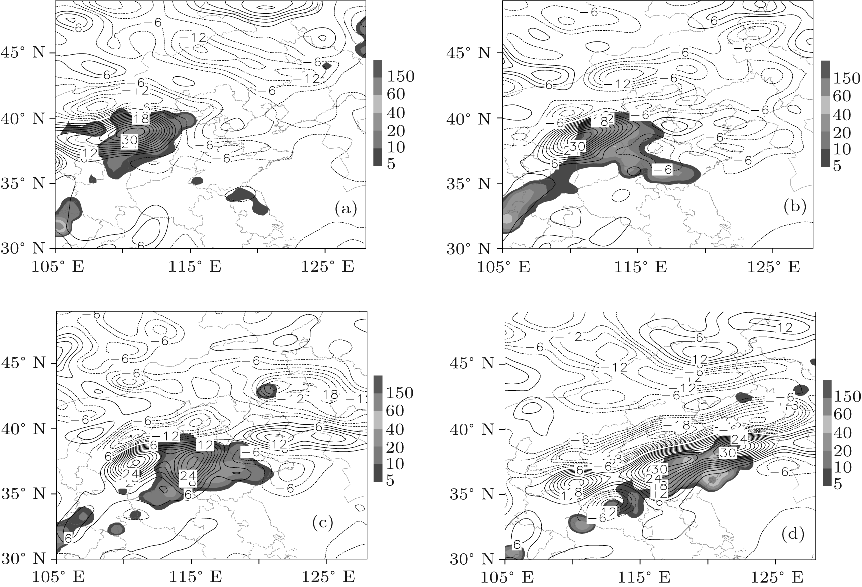	Fig.  1. The virtual pseudoenergy wave-activity density (contour, 102  kg/(m · s2)) and the observed 6-h rainfall (shaded, mm) at (a) 0000 UTC July 8, (b) 0600 UTC July 8, (c) 1200 UTC July 8, and (d) 1800 UTC July 8, 2009.

Fig.  2.

	Figure Option ViewDownloadNew Window
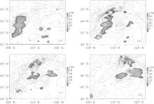
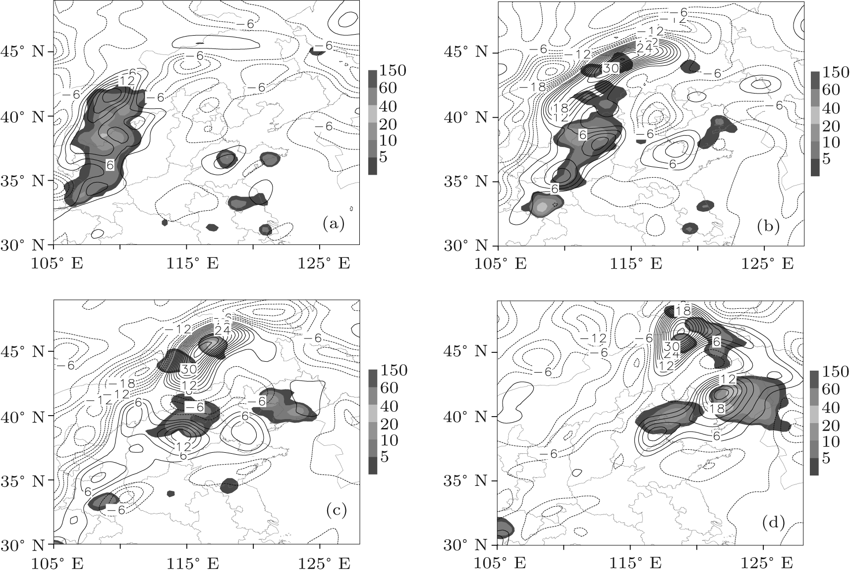	Fig.  2. The virtual pseudoenergy wave-activity density (contour, 102  kg/(m · s2)) and the observed 6-h rainfall (shaded, mm) at (a) 1200 UTC August 18, (b) 1800 UTC August 18, (c) 0000 UTC August 19, and (d) 0600 UTC August 19, 2009.

The above analysis reveals that the virtual pseudoenergy wave-activity density with positive anomaly is capable of indicating precipitation regions in the studied event. To verifies this, another heavy-rainfall event during August 18, 2009– August 19, 2009 is further investigated. In this precipitation case, the positive anomalous region of A has a dominant correspondence to the strong precipitation. They both propagate northeastwards in an analogous phase. The consistency can also be explained by the fact that the vorticity perturbation is cyclonic and the virtual potential temperature perturbation increases vertically over the precipitation region.

In this paper, the energy-Casimir method used by Haynes is employed to derive the three-dimensional virtual pseudoenergy wave-activity relation for a moist atmosphere from the nonhydrostatic primitive equations in Cartesian coordinates. The three-dimensional basic states independent of time are chosen and the Casimir function, a monotonous function of virtual potential vorticity and virtual potential temperature, is introduced in the derivation. The virtual pseudoenergy wave-activity relation obtained here is characterized by taking into account the effects of water substances, mass forcing, diabatic heating, and dissipations. Constructed in the agoestrophic and nonhydrostatic dynamical framework, the virtual pseudoenergy wave-activity relation may be applicable to diagnose the evolution and propagation of meso-scale weather systems leading to heavy rainfall.

The virtual pseudoenergy wave-activity relation does not take a local conservation form due to diabatic heating, phase change of water vapor, mass forcing, and dissipations. Besides these forces, the divergence of the virtual pseudoenergy wave-activity flux contributes to the evolution of the virtual pseudoenergy wave-activity density. The relation is valid for dry, unsaturated, and saturated atmospheres.

The virtual pseudoenergy wave-activity density is further applied to two real cases of heavy precipitation. It is revealed that the virtual pseudoenergy wave-activity density distributes in a fluctuating pattern, including positive and negative anomaly regions. The positive anomaly is capable of indicating the precipitation region because it involves the cyclonic vorticity perturbation and vertically increasing virtual potential temperature perturbation. The two factors are important dynamic and thermodynamic characteristics of precipitation.