Risk management is related to the movement of different asset prices.^{[1– 4]} The price of a financial asset is regarded as a random process, the earliest research can be traced back to Bachelier’ s work in 1900. Until the 1950s, empirical studies focused on the study of a logarithmic rate of return for time series.^{[5, 6]} In Ref.  [7], it is found that stock logarithmic returns show weak auto-correlation; however, its absolute value of the arithmetic square shows significant auto-correlation.^{[8– 12]} Recently, the difference between emerging and developed markets has been studied and the impact of financial crisis on stock price fluctuations have also been investigated.^{[13, 14]} Shen et al. used the Shanghai Stock Exchange (SSE) of Chinese 259 stocks as a sample to analyze the evolution of interaction among the plates.^[15] However, studying the volatility of financial markets in China and America, the method used in Ref.  [15] is not accurate because only the absolute values of the components of the eigenvector of the cross-correlation matrix were used to analyze the stocks.

In this paper, we try to explain more clearly the effect of the subprime crisis on the market and what kinds of changes happened in the stock prices of Chinese and American financial markets due to the subprime crisis.^{[16, 17]} The method used in our paper, which considers the negative and positive values of the component of the eigenvectors, can be used to directly observe the internal changes. We can consequently obtain different and more accurate results for the analysis of the cross-correlation matrix of the stocks.

The data is gathered from the web-site (http://www.yahoo.com). We take daily closing prices of 18 stocks from listed American banks from March 9, 2008 to August 5, 2013, corresponding to t= 1355  days. Simultaneously, we take daily closing prices of 13 stocks from listed Chinese banks from March 9, 2008 to August 5, 2013, corresponding to t= 1318  days.^[18]

In order to investigate the cross-correlation matrix among different stock prices, we first set independent time scales to measure volatility results. Let P_i(t) be the price of stock i at time t. There are 18 American bank stocks and 13 Chinese bank stocks.

The stock price return for the time interval Δ t is defined as^[19]

The renormalized volatility of the i-th stock is defined as

where is the standard deviation of R_i, and 〈 · · · 〉 represents the time average. Finally, we compute the equal-time cross-correlation matrix.^{[20, 21]} The cross-correlation C_ij between stock i and stock j is defined as

We study the eigenvalues λ and the corresponding eigenvectors u of cross-correlation matrix C = (C_ij)

where C_ii= 1. We shall analyze the cross-correlation matrix of stock price C_{13× 13}, C_{18× 18}, and C_{31× 31} corresponding, respectively, to 13 banks in China, 18 banks in America, and 31 banks in China and America.

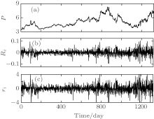
Figure  1 shows the trend of price fluctuation of the stocks of the Industrial and Commercial Bank of China. X axis represents time. The Y axes in Figs.  1(a)– 1(c) represent, respectively, the stock’ s closing price, the logarithmic return of stock price, and the renormalized return for the stocks of the Industrial and Commercial Bank of China.

Fig.  1.

	Figure Option ViewDownloadNew Window
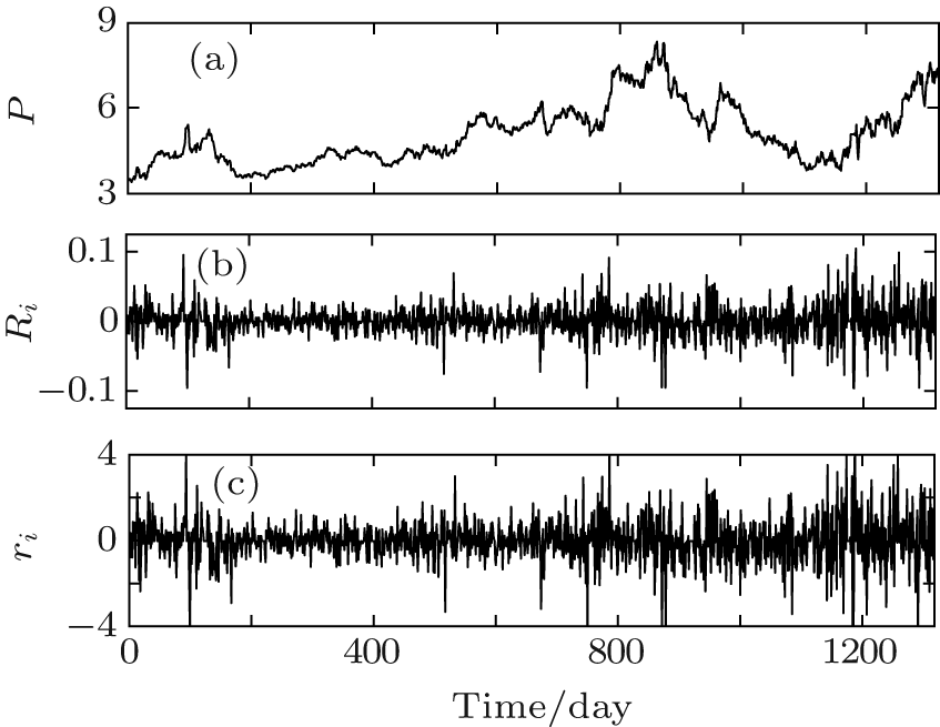	Fig.  1. Time evolution of (a) stock price Pi(t), (b) logarithmic return of stock price Ri, (c) renormalized return of stock price ri for Industrial and Commercial bank of China.

All of the components of eigenvector for cross-correlation matrix C_{13× 13}, C_{18× 18}, and C_{31× 31} are presented in Figs.  2– 5. All of the stocks used in this paper are listed in Table  1.^[22] We analyze the changes of stocks before and after the subprime crisis. In Ref.  [13], only the absolute value ∣ u_i(λ )∣ of components of eigenvector for cross-correlation matrix was considered to compare the changes before and after subprime crisis, and the differences between Chinese and American bank stocks.^{[3, 23– 25]} Based on the cross-correlation matrix eigenvector analysis of 13 stocks of Chinese market, Figure  2(b) shows the negative and positive values u_i rather than the absolute value ∣ u_i(λ )∣ for the components of the eigenvector.^{[26– 30]} This shows that some of the dominating components of the eigenvector corresponding to the second largest eigenvalue are negative. Thus, the algorithm in this paper is more accurately able to illustrate the profitability of stocks. The negative components of eigenvector could be caused by endogenous events, which are mostly are influenced by policy.^[22]

Table 1.

Table 1.

Table 1. Chinese and American bank stocks. i Company Bank Name 1 V VISA V 2 WFC Wells Fargo Company 3 ADS Alliance Data Systems Corporation 4 AIG American International Group, Inc 5 ALL The Allstate Corporation 6 AXP American Express Company 7 BAC Bank of America Corporation 8 GS The Goldman Sachs Group, Inc 9 HIG The Hartford Financial Services Group, Inc 10 JPM JPMorgan Chase Co 11 MS Morgan Stanley 12 RF REGIONS RF 13 USB U S Bancorp 14 TRV The Travelers Companies Inc 15 NYX NYSE Euronext, Inc 16 MET Met Life, Inc 17 MA MasterCard Incorporated 18 BK The Bank of New York Mellon Corporation 19 SH601998 China CITIC Bank 20 SH601166 Industrial Bank 21 SH601169 Bank of Beijing 22 SH601328 Bank of Communications 23 SH601398 Industrial and Commercial Bank of China 24 SZ002142 Bank of Ningbo 25 SH600000 Shanghai Pudong Development Bank 26 SH600015 Hua xia Bank 27 SH600016 China Minsheng Bank 28 SH600036 China Merchants Bank 29 SH601009 Bank of Nanjing 30 SH601939 China Construction Bank 31 SH601988 Bank of China

Table 1. Chinese and American bank stocks.

Fig.  2.

	Figure Option ViewDownloadNew Window
	Fig.  2. Comparison between the absolute value ∣ ui(λ )∣ algorithm by Ref.  [13] (a) and the positive and negative ui(λ ) algorithm in this paper (b). Components of eigenvectors corresponding to the largest four eigenvalues of cross-correlation matrix C13× 13 for stocks of Chinese banks from 2008– 2010 year. Here, i is the stock number.

In Fig.  3, we present the components of eigenvector corresponding to the first eight largest eigenvalues of cross-correlation matrix, where i is the stock number of 18 American listed banks and 13 listed Chinese banks.

In Figs.  3(a) and 3(b), the components of the eigenvector corresponding to the largest eigenvalue show a relatively uniform distribution pattern, which represents the market model; namely, the common interaction effect of all stocks. The eigenvectors corresponding to the second, third, and fourth largest eigenvalues show the dynamical interaction among different industry segments. We observe that for the largest eigenvalues λ ₀, all of the eigenvectors have positive component characteristics, as in Figs.  3(a) and 3(c). For eigenvectors corresponding to the second largest eigenvalue λ ₁, we find that the big component value corresponds to the stocks playing a leading role in those banks with bad enterprise benefit.^{[31, 32]}

From Figs.  3 and 4, we find that for the components of the eigenvector, if it is positive, a larger value corresponds to more rearward position in the assets rank list. The positive value component corresponds to the stock with the asset in a rearward rank position. Otherwise, for the components of the eigenvector, if it is negative, a larger value corresponds to a more forward position in the assets ranks list. The large negative value component corresponds to the stock with the asset in a front rank position.

Fig.  3.

Figure Option ViewDownloadNew Window

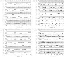
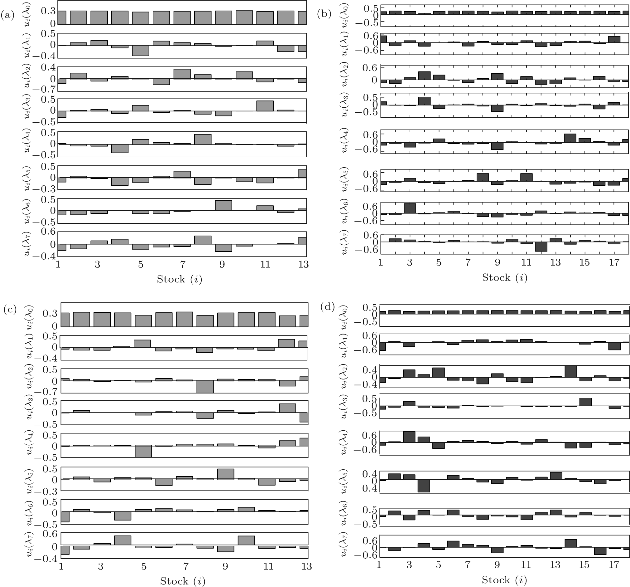Fig.  3. The eigenvectors corresponding to the eight largest eigenvalues of the cross-correlation matrix, for C13× 13 in Chinese Banks and C18× 18 in American Banks. (a) 2008– 2010 Chinese bank stocks before the subprime crisis, (b) 2008– 2010 American bank stocks before the subprime crisis, (c) 2011– 2013 Chinese bank stocks after the subprime crisis, (d) 2011– 2013 American bank stocks after the subprime crisis. Here, i is the stock number.

Fig.  4.

Figure Option ViewDownloadNew Window

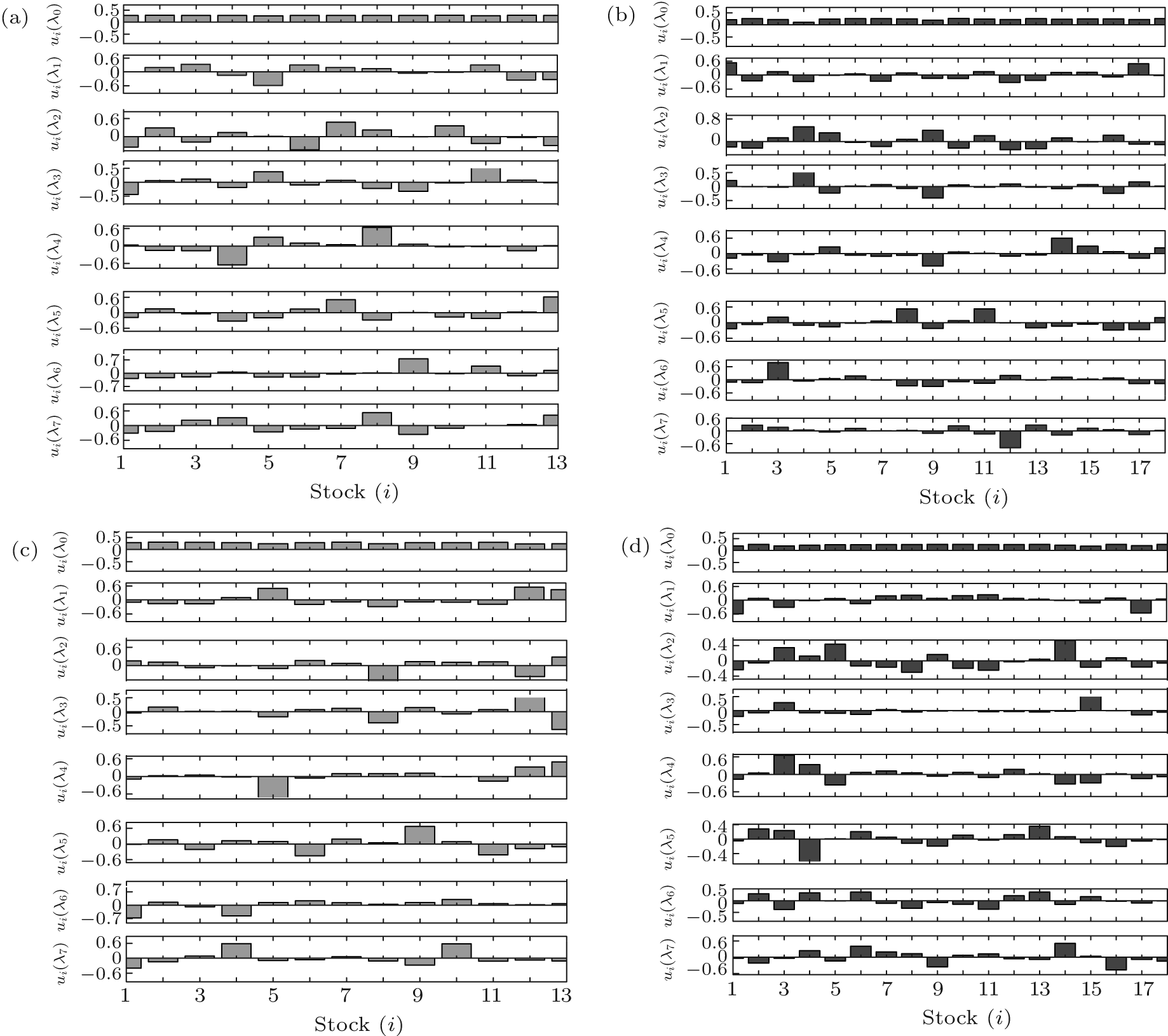Fig.  4. The positive and negative components ui(λ ) matrix C13× 13 and C18× 18 for the eigenvectors out of threshold ∣ ui∣ ≥ 0.08 corresponding to the eight largest eigenvalues of the cross-correlation matrix, where i is the stock number. (a) 2008– 2010 Chinese bank stocks before the subprime crisis, (b) 2008– 2010 American bank stocks before the subprime crisis, (c) 2011– 2013 Chinese bank stocks after the subprime crisis, (d) 2011– 2013 American bank stocks after the subprime crisis.

Fig.  5.

Figure Option ViewDownloadNew Window

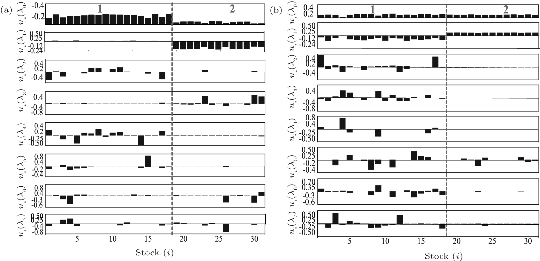Fig.  5. The positive and negative components ui(λ ) matrix C31× 31 for the eigenvectors out of threshold ∣ ui∣ ≥ 0.08 corresponding to the eight largest eigenvalues of the cross-correlation matrix, where i is the stock number. Stocks have been used in accordance with their respective countries to re-sort and divide by dotted lines. (a) 2008– 2010 American and Chinese bank stocks before the subprime crisis, (b) 2011– 2013 American and Chinese bank stocks after the subprime crisis: number 1 means American bank stocks, and number 2 means Chinese bank stocks.

As shown in Fig.  4, we introduce a threshold u_c= 0.08 to show the main components of the eigenvector. All of the component values ∣ u_i∣ ≤ u_c will be deleted. Figure  4 shows only the eigenvectors with the component value out of threshold ∣ u_i ∣ ≥ 0.08 for the largest eight eigenvalues. Figure  4 shows only the eigenvectors with the component value out of threshold ∣ u_i∣ ≥ 0.08, we see clearly the sparse distribution pattern of eigenvectors has no change before and after the subprime crises for American bank stocks; however, it changes from sparse to dense for Chinese bank stocks.

In Fig.  5, we present the interactions among a total of 31 stocks for the American market and Chinese market. We present the eigenvector of cross-correlation matrix C_{31× 31} for 31 stocks contained in the Chinese market and American market. Hence, this figure more clearly shows that the distribution pattern for eigenvectors has no change before and after subprime crises for American bank stocks; however, it changes from sparse to dense for Chinese bank stocks.

Based on the closing price of stocks for Chinese and American banks, and the cross-correlation matrix for stocks, we analyze the effect due to the subprime crisis in the financial markets. We set a threshold to select the dominating components of eigenvectors to observe the changes that happen before and after the subprime crisis. From the cross-correlation matrix analysis, we find that the stock prices in the emerging market are more correlated than that in the developed market. By considering the component value of the eigenvector to be positive or negative, and keeping only the component value out of the threshold, we can more clearly show the distribution pattern changes for the eigenvector before and after the subprime crises. Hence, the cross-correlation interaction in the markets can be seen more clearly.