

Evaluation of influences of frequency and amplitude on image degradation caused by satellite vibrations*
[Nan Yi-Binga), b) , Tang Yia), b)†  , Zhang Li-Jun
a), b) , Zheng Chenga), b) , Wang Jinga), b) ]
, Zhang Li-Jun|
|


†Corresponding author. E-mail: tangyi4510@bit.edu.cn
*Project supported by the National Basic Research Program of China (Grant No. 2013CB329202) and the Basic Industrial Technology Project of China (Grant No. J312012B002).
Satellite vibrations during exposure will lead to pixel aliasing of remote sensors, resulting in the deterioration of image quality. In this paper, we expose the problem and discuss the characteristics of satellite vibrations, and then present a pixel mixing model. The idea of mean mixing ratio (MMR) is proposed. MMR computations for different frequencies are implemented. In the mixing model, a coefficient matrix is introduced to estimate each mixed pixel. Thus, the simulation of degraded image can be performed when the vibration attitudes are known. The computation of MMR takes into consideration the influences of various frequencies and amplitudes. Therefore, the roles of these parameters played in the degradation progress are identified. Computations show that under the same vibration amplitude, the influence of vibrations fluctuates with the variation of frequency. The fluctuation becomes smaller as the frequency rises. Two kinds of vibration imaging experiments are performed: different amplitudes with the same frequency and different frequencies with the same amplitude. Results are found to be in very good agreement with the theoretical results. MMR has a better description of image quality than modulation transfer function (MTF). The influence of vibrations is determined mainly by the amplitude rather than the frequency. The influence of vibrations on image quality becomes gradually stable with the increase of frequency.
As the satellite orbits the earth, complex motion errors of the platform, including vibrations, are ubiquitous. Information of the scene coming from different sub-areas will be aliased on a given pixel, which will lead to serious degradation of remote sensing images.
The influence of vibrations on imaging quality has been widely investigated over the last decades. In Refs. [1]– [6], the effects of vibrations on different kinds of imageries are modeled by the calculation of modulation transfer function (MTF). However, MTF analysis does not take into consideration the relationship between satellite vibrations and practical acquired images. Thus, it cannot provide integral model of actual image degradation. In addition, the sampling time of astronautic remote sensor and the frequency of vibration vary in a large range, so the value of te/T0 far exceed its research range.
There are two common assumptions in previous research: (1) low-frequency vibration has a larger amplitude while high-frequency vibration has a smaller amplitude; (2) the influence introduced by low-frequency vibrations is more serious.[2] However, the launch of satellites in recent years with higher resolution has weakened these assumptions, resulting in more serious image degradation. More importantly, the exposure times of actual remote sensors differ greatly, so a certain frequency that is low for some sensors may be high for other ones. Based on the above mentioned two reasons, it is necessary to separate the influence of vibration frequency from that of amplitude, and quantitatively study them separately, and then the relationship between the extent of pixel mixing and vibration parameters can be obtained.
In this paper, we analyze and model the process of image degradation caused by satellite vibration. The relationship between vibration parameters and degraded image is set up. We calculate the mean mixing ratio (MMR) for vibrations with different attitudes and frequencies. The simulated degraded images can be obtained by using these results. Finally, ground experiments are carried out to verify the theory.
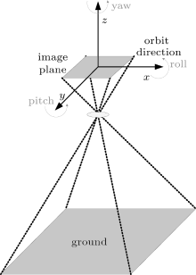
In space domain, vibration of satellite shows 6 degrees of freedom, which can be reduced to translations and rotation along 3 coordinates. Rotations are the main factor that leads to image degradation.[7] As shown in Fig. 1, we define those rotations as the roll, the pitch and the yaw respectively.
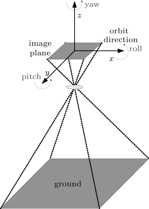 | Fig. 1. Motion and rotation model of satellite. |
In frequency domain, according to the ratio of exposure time te to the vibration period T0, satellite vibrations are divided into low frequency and high frequency. The low vibration frequency case involves te/T0 ≤ 0.25, and is equivalent to uniform linear motion. When te/T0 > 0.25, the vibrations belong to high-frequency case, and can be regarded as sinusoidal motion. [8]
Generally, the amplitude of vibration declines with the increase of frequency. Therefore, the higher frequency vibrations possess smaller vibration amplitude, and the frequency can reach a value of over 1000 Hz.[9] However, the energy of vibration is mainly concentrated in a range of 0– 200 Hz.[10, 11] Actual vibrations are random and complicated, which may involve different frequencies and amplitudes at the same time.
The essence of exposure progress for an astronautic imaging device is an energy accumulation. Therefore, the sampling of each pixel of the sensor can be understood as an overlay of integral and discretely sampling. Image points will move along a path, if relative motion between satellite and scene exists during all the acquisition procedure. One can divide the exposure time into N slices. When N grows big enough, the motion during every time slice can be regarded as a uniform linear motion so that

where g(x, y) denotes the captured image and f(x − Δ x(t), y − Δ y(t)) the clear image shifted by original image f(x, y), in which (Δ x(t), Δ y(t)) expresses the image displacement at time t. We set Δ x(t) = md + x′ , Δ y(t) = nd + y′ , where d denotes the pixel size, m, n ∈ [0, N], and they have the same signs as x′ and y′ respectively. Actual mixing pixels are (i + m, j + n) combined with its adjacent 8 pixels. Thus, at time t, mixed pixel g(i, j) can be write as

where ku, v is the ratio of original clear pixel overlapped by shifted pixel, which may be expressed by a coefficient matrix
Considering the shifted pixel may cover 4 pixels at most at the same time, let ω x and ω y be the sign of x′ and y′ , we define two signed variables ξ and η as | x′ /d| and | y′ /d| , so that K may be expressed as the product of the corresponding elements of W and A
As mentioned above, given the satellite rotations of a moment, one can work out the pixel displacement. From Eqs. (2)– (5), the intensity of the pixel is obtained. The total intensity in exposure time may be calculated by Eq. (1).
After substituting Eq. (2) into Eq. (1), the resulting equation may be written in the form of
At this point, one may find that 
The spatial resolution of current satellite sensors with high resolution and currently in use is about 1 m, and their orbital altitudes are beyond 600 km generally. The attitude stability of their spacecraft could achieve 10− 1– 10− 3 arcsec/s, [12– 16] which means that the image displacement caused by satellite vibrations falls within a pixel. An actual image pixel is mixed by its adjacent 8 pixels such that m, n = 0 in Eqs. (2) and (3).
In this paper, we take the pitch attitude as an example to analyze the influence of satellite vibrations. Let the focal length of imaging system be f, and the rotation of pitch Δ α . The influence of pitch is parallel to the direction of Δ x, and approximately Δ x(t) = fΔ α (t). To simplify the calculation, we assume that the mixed pixels are (i, j) and (i + 1, j) during all the exposure, such that Δ x(t) > 0 and Δ y(t) = 0. Combining Eqs. (3)– (5), then coefficient matrix K may be written in a different form as
Assuming the pitch rotation at time t

where α max is the max attitude jitter of pitch, and φ is the initial phrase, the MMR of pixel (i + 1, j) under vibration of pitch is obtained as
Let te/T0 = N + s, where N denotes an integer greater than or equal to 0, and s a decimal between 0 and 1, then equation (9) will be written in the following form:

The value of

changes over the initial phrase φ and te/T0. Its average value can be obtained by integration
which reveals that the MMR of pixel (i + 1, j) reaches its minimum when te/T0 = 1, in which case MMR = α maxf/(2d).
The average of MMR can be express in the form of

It is obvious that the more the vibration amplitude is, the more serious the pixel mixing is. Figure 2 shows the curve of
 | Fig. 2. Curve of |
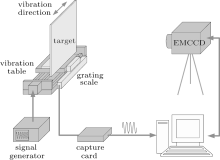
As shown in Fig. 3, the ground simulation system consists of a motion signal generator, a translation stage with a simulated ground target on it, a grating scale, a digital capture card and a camera of EMCCD (Mode: ProEM512 of Princeton Instruments, resolution ratio: 512 × 512, pixel size: d = 16 μ m, 16-bit digitization). The focal plane of the camera is parallel to the target. The signal generator can export vibration signal to control the position of the translation stage at different moments. One can set attitude, frequency and amplitude of the vibration signal. Then the signal is transferred to the translation stage. With the vibration, displacement of the motion is captured by the grating scale and capture card in real-time, then the vibration curve is displayed. By adjusting the vibration parameters, sinusoidal vibration can be realized. At the same time, images of the target are taken by the EMCCD. In the experiments, the EMCCD is set to be in the frame transfer mode, the transfer time is 0.3 ms per frame, and the readout rate is 5 MHz. To exclude the influence of EMCCD configuration, each exposure is manually controlled. During the exposure, the vibration mode is kept unchanged. The distance between camera and target is 2 m, and the focal length f = 100 mm.
We present experimental results under two kinds of vibration conditions: different vibration amplitudes with the same vibration frequency and different vibration frequencies with the same vibration amplitude. We take two groups of images with and without vibration for each kind of condition. Then the differences between the two groups are evaluated by mean square error (MSE) and peak signal noise ratio (PSNR). They are defined respectively as follows:

where M and N denote the image size. To exclude the influence of the randomness of image acquisitions, multiple images are taken and averaged for every vibration model especially for the very low frequency vibrations.
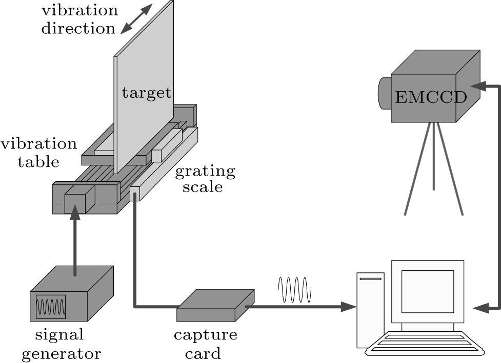 | Fig. 3. Vibration imaging simulation system, where the vibration table is driven by the signal generator, the grating scale captures the motion in real-time, and degraded images are taken by the EMCCD in the mean time. |
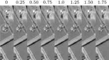
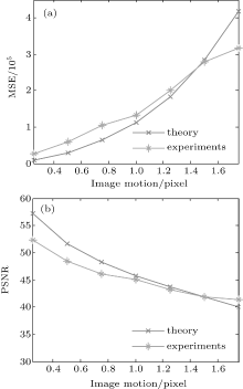
The experiments are carried out under the same value of te/T0 equal to 1. The exposure time te = 200 ms, which means the real vibration frequency is 5 Hz. The image motion varies from 0 to 1.75 pixel. The experimental and theoretical results can be seen in Figs. 4 and 5. It is obvious that under the same vibration frequency, the effects become serious as the vibration amplitude increases. When the image motion reaches 0.75 pixel, the MSE of degraded image is about 29 times that of the image without vibration. The PSNR declined more than 24%.
Compared with the images without vibration, the degrees of change of MSE and PSNR can be seen in Table 1. The image quality is greatly influenced by the vibration amplitude.
 | Fig. 4. Parts of degraded images, with the image motion varying from 0 to 1.75 pixel. |
 | Fig. 5. Theoretical and experimental MSE (a) and PSNR (b) variations for different amplitudes of vibration with the same vibration frequency. |
| Table 1. Change degrees of MSE and PSNR. |
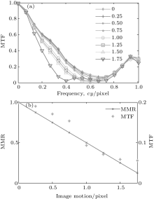
To find the influence of vibration on MTF of the imager, we calculate the values of MTF of different images by knife-edge method. Figure 6(a) shows the variations of MTF for different amplitudes of vibration with the same vibration frequency. Figure 6(b) shows the values of MMR of initial pixel and the value of MTF at half sampling frequency changing with vibration amplitude. It can be seen that the image quality deteriorates seriously with the increase of vibration amplitude. The results of MMR and MTF analysis have a strong resemblance to MSE and PSNR evaluations.
 | Fig. 6. MTF of images (a) and MMR for different vibration amplitudes of vibration (b) with the same vibration frequency. |
In this case, considering various sampling times of satellite imagery that is used in remote sensing, our experiments are divided into two parts, i.e., the low-frequency part and the high-frequency part. The low-frequency part involves sampling time te shorter than the vibration period T0, and the high-frequency part involves te ≥ T0. For the low-frequency case, the value of te/T0 varies from 0.05 to 1 (te = 100 ms, the real vibration frequency varies from 0.5 Hz to 10 Hz), while te/T0 varies from 1 to 20 (te = 2000 ms, the real vibration frequency varies from 0.5 Hz to 10 Hz) for the high-frequency case. The vibration amplitudes are 40, 80 and 160 μ rad (equivalent to 0.5, 1 and 2 pixel of max image motion) for both.
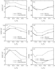
We calculate the theoretical MMR of mixed pixel, then, obtain the degraded images of simulation by Eq. (6) as the theoretical data. The experimental and theoretical evaluation results of MSE and PSNR for low-frequency part can be seen in Tables 2 and 3 and Fig. 7. Tables 2 and 3 show the values of MSE and PSNR without vibration, average image degradations for different frequencies and differences between the maximum and minimum of image degradation. Take the case of image motion equal to 1 pixel as an example, while in the case without vibration, MSE = 3701 and PSNR = 61. When vibration exists, images are seriously degraded. The average change of MSE is more than 44 times, and the PSNR decreases by 23% on average. It can also be seen in Fig. 7 thant, for all amplitudes of vibration, with the increase of te/T0, the image quality first decreases and then gradually rises. However, the differences between the maximum and minimum of MSE and PSNR are small compared with the average value of degradation. It means that although the influence of vibration fluctuates with frequency, the effect of frequency on the image degradation is limited. According to the theoretical analysis of MMR in Section 3.2, with the changing of vibration frequency, the average value of image motion varies, leading to the fluctuation of MMR. Therefore, essentially, the influence of frequency on image degradation is realized by changing the mean image motion during the exposure. And this variation can be denoted by MMR.
| Table 2. Change degrees of MSE. |
| Table 3. Change degrees of PSNR. |
 | Fig. 7. Theoretical and experimental MSE and PSNR variations with te/T0 for the case of te/T0 ≤ 1. (a) MSE, 0.5 pixel; (b) PSNR, 0.5 pixel; (c) MSE, 1 pixel; (d) PSNR, 1 pixel; (e) MSE, 2 pixel; (f) PSNR, 2 pixel. |
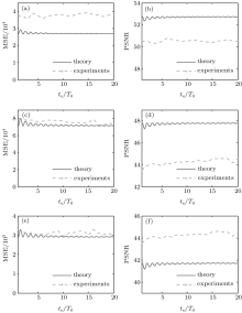
The experimental and theoretical evaluation results of MSE and PSNR for high-frequency part are shown in Tables 4 and 5 and Fig. 8. Results indicate that when the exposure time is longer than the vibration period, the image quality also declines apparently. When te/T0 increases, the fluctuation of image degradation decreases. However, it tends to be less volatile with the change of frequency for all amplitudes of vibration, which are very smaller than the results of the low-frequency case. This phenomenon is also in accordance with the MMR theoretical result.
| Table 4. Change degrees of MSE. |
| Table 5. Change degrees of PSNR. |
The overall trend of experimental results becomes better as te/T0 increases, because noise and other motion errors exist in actual vibrations. The bigger the value of te/T0 is, the less the influence of the motion errors is.
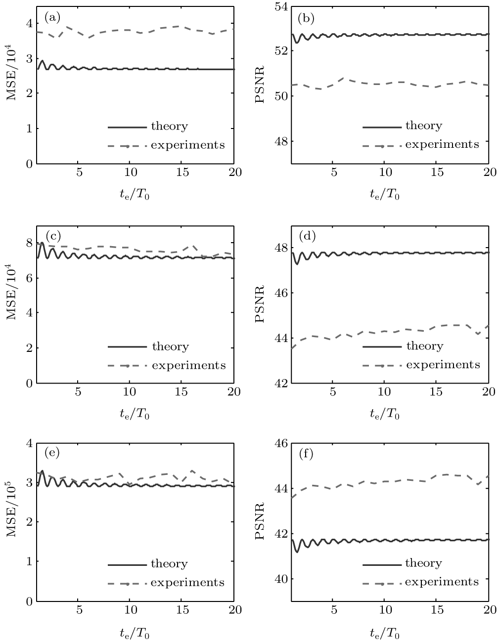 | Fig. 8. MSE and PSNR variations of experimental images with te/T0 for the case of te/T0 ≥ 1. (a) MSE, 0.5 pixel; (b) PSNR, 0.5 pixel; (c) MSE, 1 pixel; (d) PSNR, 1 pixel; (e) MSE, 2 pixel; (f) PSNR, 2 pixel. |
Through the above results and discussion, we can find that either for low-frequency case or high-frequency case, the experimental variation trend of image quality is consistent with theoretical result. To provide an intuitive expression of this conformity, we combine the two groups of experimental data in Figs. 7 and 8, for those data are obtained separately and divided according to te/T0 = 1. After comparing the values when te/T0 = 1 in the two groups of data, the weight factor is calculated. Then the two groups of data are weight-processed, and the treated two groups of data merge into one group of data. For instance, we contrast the matching MSE curve with the
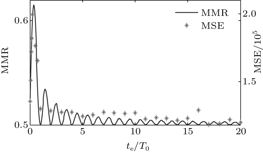 | Fig. 9. Comparison between the experimental and theoretical results of MSE. |
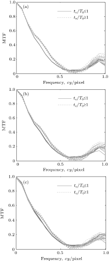
The values of MTF for different vibration frequencies are also computed and shown in Fig. 10. For the 3 vibrations under different frequencies, the values of MTF all show small variations under the same amplitude despite the changing of frequency. This phenomenon is different from the scenarios with the variation trend of MMR and MSE in Fig. 9. It means that the degree of image degradation is determined primarily by the amplitude of vibration, and the MTF calculation cannot reveal the subtle difference in image quality.
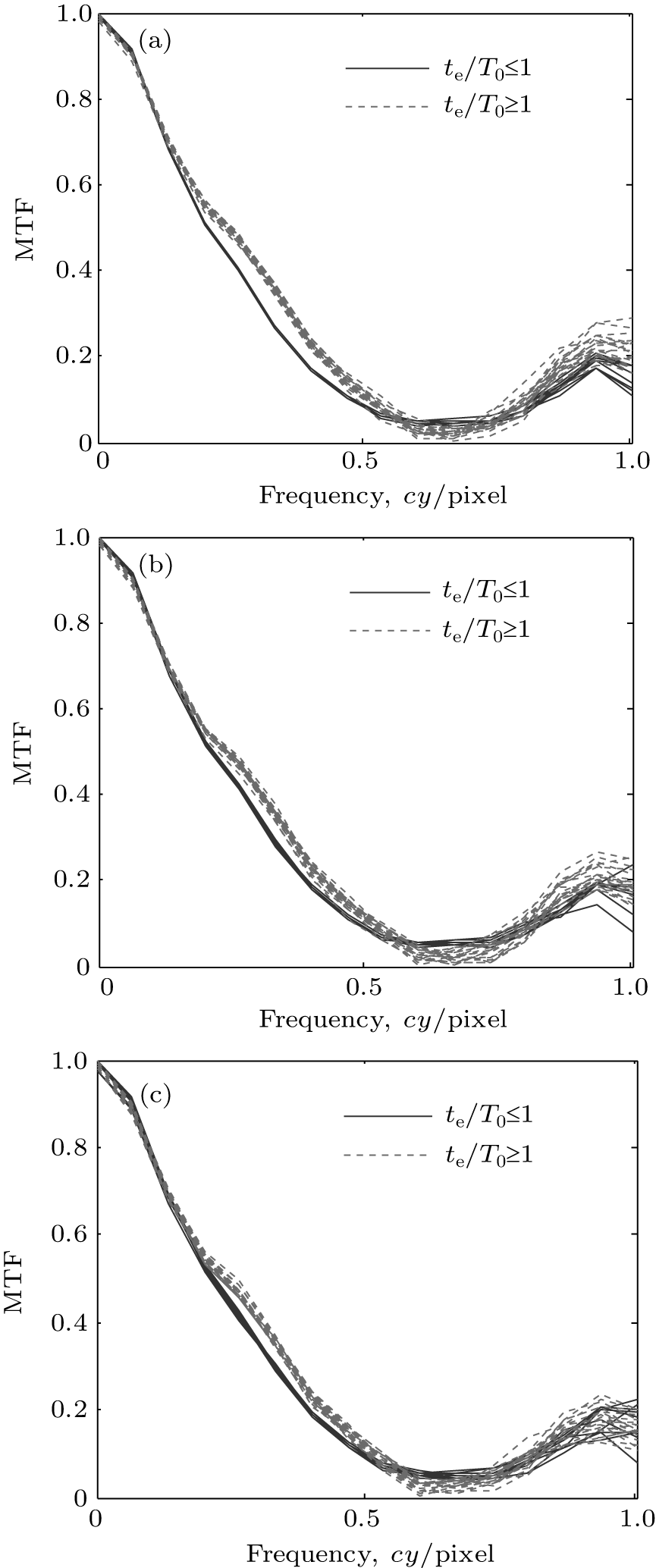 | Fig. 10. Variations of MTF of images with vibration frequency for the case with the same amplitude. (a) 0.5 pixel, (b) 1 pixel, (c) 2 pixel. |
We have characterized the vibration principles of satellite and modeled the progress of image degradation. In the proposed model, the relationship between vibration parameters and motion displacement is established by using a coefficient matrix. The originality of our work is to present the idea of mean mixing ratio. When the attitude parameters of the satellite are given, the degraded image can be obtained. Furthermore, MMRs for different frequencies and amplitudes of vibration are deduced. We also carry out experiments to verify the different effects of vibration parameters. Results of the simulated experiments show that image quality suffered a serious decline while vibrations exist. Under the same amplitude, the image quality experiences a progress of first decrease and then increase to steady as the vibration frequency increases. Under the same vibration frequency, the influence of vibrations becomes worse with the increase of amplitude. These results mean that the influence of vibration amplitude on image quality is far more important than that of vibration frequency. The vibration amplitude determines the degree of degradation of an actual remote sensing image. The experimental results also reveal that the MMR evaluation can better respond to image deterioration than MTF analysis. Although the amplitude of high-frequency vibration is relatively small, more attention should be paid to the improvement of resolution of remote sensors. For isolating vibration design and image restoration, the specifications of different imaging systems should be taken into account.
| 1 |
|
| 2 |
|
| 3 |
|
| 4 |
|
| 5 |
|
| 6 |
|
| 7 |
|
| 8 |
|
| 9 |
|
| 10 |
|
| 11 |
|
| 12 |
|
| 13 |
|
| 14 |
|
| 15 |
|
| 16 |
|