


Precision spectroscopy with a single 40Ca+ ion in a Paul trap*
[Guan Huaa), b) , Huang Yaoa), b) , Liu Pei-Lianga), b) , Bian Wua), b), c) , Shao Hua), b), c) , Gao Ke-Lina), b)†  ]
]
]


†Corresponding author. E-mail: klgao@wipm.ac.cn
*Project supported by the National Basic Research Program of China (Grant Nos. 2012CB821301 and 2005CB724502), the National Natural Science Foundation of China (Grant Nos. 11474318, 91336211, and 11034009), and Chinese Academy of Sciences.
Precision measurement of the 4s2S1/2–3d2D5/2 clock transition based on40Ca+ ion at 729 nm is reported. A single40Ca+ ion is trapped and laser-cooled in a ring Paul trap, and the storage time for the ion is more than one month. The linewidth of a 729 nm laser is reduced to about 1 Hz by locking to a super cavity for longer than one month uninterruptedly. The overall systematic uncertainty of the clock transition is evaluated to be better than 6.5×10⁻¹⁶. The absolute frequency of the clock transition is measured at the 10−15 level by using an optical frequency comb referenced to a hydrogen maser which is calibrated to the SI second through the global positioning system (GPS). The frequency value is 411 042 129 776 393.0(1.6) Hz with the correction of the systematic shifts. In order to carry out the comparison of two40Ca+ optical frequency standards, another similar40Ca+ optical frequency standard is constructed. Two optical frequency standards exhibit stabilities of 1×10⁻¹⁴ τ−1/2 with 3 days of averaging. Moreover, two additional precision measurements based on the single trapped40Ca+ ion are carried out. One is the 3d2D5/2 state lifetime measurement, and our result of 1174(10) ms agrees well with the results reported in [Phys. Rev. A62 032503 (2000)] and [Phys. Rev. A71 032504 (2005)]. The other one is magic wavelengths for the 4s2S1/2–3d2D5/2 clock transition; λ| mj|=1/2= 395.7992(7) nm and λ| m j|=3/2 = 395.7990(7) nm are reported, and it is the first time that two magic wavelengths for the40Ca+ clock-transition have been reported.
Accurate time and frequency standards have many applications such as the realization of the SI base units of time, satellite-based navigation, and tests of physical theories. Since 1967, the definition of the SI second is based on the ground hyperfine transition of the 133Cs atom. Currently the Cs fountain clock with the smallest uncertainty ever reported is 2.3× 10− 16.[1] With high-Q transitions, the optical frequency standards based on laser-cooled trapped ions or atoms can achieve even better stability and accuracy. Optical frequency standards have been developed rapidly thanks to recent techniques using cold atoms, optical frequency combs, [2, 3] and ultra-narrow linewidth lasers.[4, 5] Optical frequency standards have been developed rapidly in recent years based on ultracold neutral atoms or single ions such as Sr, [6– 9] Yb, [10] Sr+ , [11, 12] Yb+ , [13, 14] Hg+ , [15] Al+ , [15, 16]40Ca+ .[17– 19] Uncertainty on the order of 10− 18 is reported with Sr[6] and Al+ .[16] The best evaluation of the frequency uncertainty reported so far is 6.4× 10− 18 with Sr.[6] And the stability has reached 3× 10− 18 at 10 000 s for Sr[6] and 1.6 × 10− 18 after only 7 h of averaging time for Yb, [10] respectively. The uncertainties and stabilities evaluated above, both based on single trapped ions or ultracold neutral atoms, have already surpassed those of the best Cs fountain clocks. They are expected to take the place of the Cs primary microwave standard as the definition of the SI second in the near future, and the optical transition frequency of some atoms, ions and molecules were recommended by the International Committee for Weights and Measures (CIPM) as secondary representations of the second, contributing to International Atomic Time (TAI).[20]
In China, many institutes are pursuing research in optical frequency standards, with ultracold neutral atoms or single ions such as Sr, Yb, Ca, Hg, Al+ , Ca+ , Hg+ , In+ , and Ba+ being developed. For instance, recently Xu et al. proposed reducing the inhomogeneous-excitation frequency shift at the 10− 19 level and presented a detailed experimental study of the clock-transition spectrum of the ytterbium optical lattice clocks.[21, 22] And there are some suggestions for an active optical clock.[23, 24]
As there are commercially available lasers for photoionization, cooling, manipulation, and detection, the Ca+ ion has been chosen for building a practical optical clock, which may be an alternative candidate for the new definition of the SI second.[25] The optical frequency standard based on a single Ca+ ion is being developed by the Quantum Optics and Spectroscopy Group in Innsbruck, [17] the National Institute of Information and Communications (NICT) in Japan, [18] and the Physique des Interactions Ioniques et Molecularies in France.[26] And the odd isotope of the 43Ca+ ion can be used as an optical frequency standard, because it is immune to the first-order Zeeman frequency shift.[27] The 40Ca+ is also popular in atomic physics and quantum information.[28– 30]
In this paper, the experimental work on the development of the optical frequency standard based on a single 40Ca+ ion at Wuhan Institute of Physics and Mathematics (WIPM), the Chinese Academy of Sciences (CAS) is introduced. First, the 40Ca+ optical frequency standard is described, including ion trap and laser systems, and the experimental results, including single trapped and laser-cooled Ca+ ions, locking the 729 nm clock laser’ s frequency to the Ca+ ion, evaluating the systematic shifts and uncertainties of the clock transition and measuring the absolute frequency of the clock transition using an optical frequency comb referenced to a hydrogen maser calibrated to the SI second through the global positioning system (GPS). Then, a comparison of two 40Ca+ optical frequency standards is presented, including the principles, the processes, and the results. Last, a summary and an outlook are given.
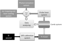
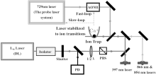
A 40Ca+ optical frequency standard is composed of three parts, the first is the physical system, including Paul trap, cooling laser, and repumping laser. The second is the probe laser with ultra narrow linewidth, and the last one is the optical frequency comb used for measuring the absolute frequency of optical frequency transition. The overall schematic diagram of the experimental setup is shown in Fig. 1. In the following parts, we will describe the experimental setup and results of our 40Ca+ optical frequency standard.
 | Fig. 1. Overall schematic diagram of the experimental setup. |
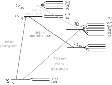
A partial energy level diagram of 40Ca+ is shown in Fig. 2. The lifetime of the 3d2D5/2 state is about 1.1 s and the linewidth of the 4s2S1/2– 3d2D5/2 electric quadrupole transition is about 0.14 Hz.[31, 32] In our lab, a single 40Ca+ ion is trapped and laser-cooled in a miniature electric quadrupole Paul ring trap.[33– 37]
 | Fig. 2. Partial energy level diagram of 40Ca+ showing the principal transitions used in cooling, repumping and probing of the reference 729 nm transitions. |
The ion trap is composed of a ring and two endcap electrodes in our experiment. The diameter of the ring is r0 = 0.8 mm, and the distance of the endcap to center is z0 = 0.7 mm. Two compensation electrodes perpendicular to each other are set in the ring plane to compensate for the ion’ s excess micromotion, and the distance from either of these two electrodes to the center is 5 mm. The miniature structure is beneficial for confining a single ion in the Lamb– Dicke regime to eliminate the first-order Doppler shift; the nonstandard configuration (compared to the classical Paul trap) can reduce background noise and increase the S/N ratio. The trap is enclosed in a chamber that is evacuated to a pressure of less than 10− 8 Pa.
A trapping rf field with an amplitude 580Vp– p is applied to the ring at the frequency of 9.8 MHz. The excess micromotion is nulled by precisely adjusting the voltages on the endcap and compensation electrodes.
Because the nuclear spin of 40Ca+ is 0, there is a first-order dependence between the S1/2– D5/2 transition frequency and the magnetic field. Variation of the ambient magnetic field strongly affects the precision of the optical frequency standard. As the transition frequency changes due to the linear Zeeman effect and the transition linewidth can be broadened to 10– 100 times, double layer magnetic shields are installed outside the ion trap vacuum chamber to shield the variation of the ambient magnetic field, and an attenuation factor of about 200 is achieved. A stable dc magnetic field of less than 1 μ T is applied after compensating the residual field by three pairs of coils perpendicular to each other with three individual current supplies (YL4010& YL4012, Yltec).
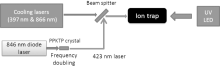
In early experiments in our Lab, the 40Ca+ ions were loaded by ionizing the neutral Ca atom beam with electron bombardment. This method is effective for loading ions. However, there are two main disadvantages. The first is the uncontrollable number of ions, and the second is that lots of electrons will attach on the electrodes and affect the ion storage. Recently photon ionization is applied with highly efficient loading by using a two-step photo-ionization scheme on a weak thermal beam of neutral atomic calcium.[38] The schematic diagram for ion loading and laser cooling is shown in Fig. 3. A custom-made Littrow configuration diode laser is used to produce a 846 nm laser with power of about 100 mW, the laser beam is focused into a 5-mm-long PPKDP crystal and frequency doubled with the second-harmonic generation (SHG), and the power of the 423 nm laser produced is about 10 μ W. The 423 nm laser beam is focused into the ion trap together with a UV LED to carry out the photon ionization.
 | Fig. 3. Schematic diagram of ion loading and laser cooling. |
To realize an optical frequency standard, trapping steadily and cooling effectively a single Ca+ ion in a Paul trap is an important prerequisite. Two lasers are needed in the process. One is a 397 nm cooling laser which pumps the ion from the 42S1/2 to the 42P1/2 level. The other is 866 nm radiation to drive 32D3/2– 42P1/2 transition for avoiding the ion staying at the 32D3/2 metastable level and stopping the cooling cycle.
The 397 nm laser is generated by a commercial diode laser (DL100, Toptica). In typical experimental conditions (T = 23.6 ° C, I = 61 mA), the output power of the laser is about 30 mW. Its linewidth is about 4 MHz, and the long-term drift is about 300 MHz in 30 minutes. In order to reduce the linewidth of the laser, we lock the laser to the transmission peak of a confocal Fabry– Perot interferometer with temperature stabilization (FPI100, Toptica). The free spectrum range (FSR) is 1 GHz, and its finesse is about 400. In this way, the linewidth of the 397 nm laser is reduced to below 1 MHz, which is narrow enough for laser cooling of 40Ca+ , since the natural linewidth of 42S1/2– 32P1/2 transition is ∼ 22.3 MHz. When we monitored the long-term drift of the 397 nm laser with an optogalvanic (OG) signal, we found the laser still drifts several hundreds of MHz within 30 mins. Then, we used the OG signal as a reference to control the cavity length of the FPI100 by a computer program. Thus, the long-term drift of the laser is reduced to below 10 MHz within 2 h.[39] The method for frequency stabilization of the 866 nm laser is similar.
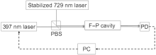
However, to achieve the long-time-running of the optical frequency standard, 397 nm laser is stabilized to a stable 729 nm laser by transfer cavity scheme, [40] see Fig. 4. As the reference, the 729 nm laser’ s performance is a key. We will describe the frequency stabilization of the 729 nm laser in detail in the following section. The transfer cavity is a custom-made plane-concave cavity, and its finesse is more than 50 for both the 397 nm and 729 nm lasers. The scanning frequency is 100 Hz recurrence to a PZT, and the 397 nm and 729 nm transmission light of the cavity is detected by two photo diodes (PD) respectively. The signals from the two PDs are then amplified and acquired by a computer using an analog to digital convertor (ADC). By comparing the transmission fringes of the 397 nm and 729 nm lasers, the relative drift rate of the 397 nm laser with respect to the 729 nm laser can be deduced. At the same time, the error signal is fed back to the 397 nm laser to stabilize the laser’ s frequency. In this way, the frequency drift is reduced to less than 1 MHz in few hours.
 | Fig. 4. The 397 nm laser stabilization by a transfer cavity. |
The 866 nm repumping laser’ s frequency stabilization employs a similar method. The difference is that the transfer cavity is a commercial cavity (FPI750, Toptica) and the long-term drift of the 866 nm laser is reduced to less than 1 MHz in few hours.
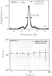
To observe the high-Q optical clock transition with a natural linewidth of 0.14 Hz, the 729 nm probe laser’ s linewidth is expected to be at Hz level or even sub-Hz level. A commercial Ti:sapphire laser (MBR-110, Coherent) is adopted. The Ti:sapphire laser’ s wavelength can be adjusted continuously in a large range and is very stable when locked. It is locked to a super cavity using the Pound– Drever– Hall (PDH) technique.[41] In a previous experiment, a Zerodur cavity was adopted.[33– 37, 39] Later, a ULE cavity replaced the Zerodur cavity. The length of the ULE cavity is 10 cm with the finesse > 200000, and the cavity is placed on an active isolated platform (TS-140, Table Stable). Meanwhile two layers of temperature control and acoustic isolation are constructed to isolate the effect of the system from its surroundings. In order to measure the linewidth and the long-term drift of the 729 nm laser, the heterodyne beatnote of the Ti:sapphire laser and another 729 nm diode laser locked to a similar ULE cavity is adopted, and the result is about 1 Hz (see Fig. 5(a)). If the linewidths of the two lasers are comparable, one can deduce the linewidth of each laser less than 1 Hz. After the linear drift of ∼ 31 mHz is removed, the Allen deviation of the two lasers is about 1.5 Hz (1– 100 s), and the stability of each laser is about 1 Hz (1– 100 s).
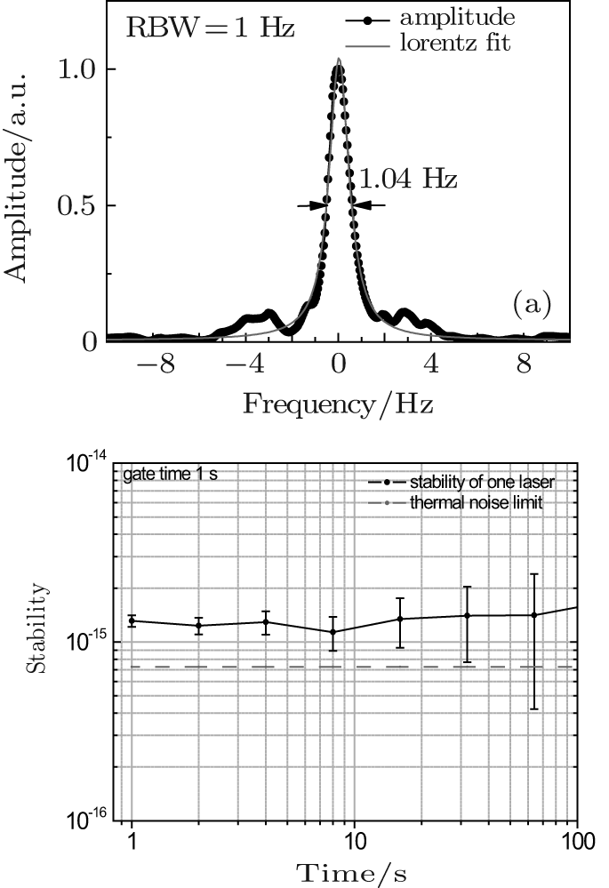 | Fig. 5. (a) A 1 Hz linewidth beatnote of the Ti:sapphire laser and the diode laser; (b) the beatnote stability of two locked lasers. |
To measure the frequency of the clock transition, a femtosecond optical frequency comb (fs comb)[42, 43] (FC 8004, MenloSystems) was used and referenced to a hydrogen maser (Fig. 6). A mode-locked Ti:sapphire laser pumped by 5 W laser at 532 nm (Verdi V-6, Coherent) produced fs pulses (normally 30 fs) at a repetition rate of approximately 200 MHz. The frequency of the n-th comb component can be expressed as fn = nfrep + fCEO, [44, 45] where frep is the repetition rate of the laser pulses and fCEO is the carrier-envelope offset frequency. The output is focused into two pieces of photon crystal fiber (PCF): one is for the observation of the offset frequency detection, and the other is for the probe laser measurement. The spectrum range is normally broadened to over an octave after the fiber, from approximately 500 nm to 1100 nm. A self-referencing system with an f-to-2f interferometer is introduced for the offset frequency detection. The infrared part of the broadened comb beam is separated with a dichroic mirror and the frequency is doubled with the SHG using a 5-mm-long KNbO3 crystal, and then overlapped with the frequency-broadened green beam using a polarized beam splitter (PBS). The signal to noise ratio (S/N) of the carrier-envelope beat frequency is 40 dB at a resolution bandwidth of 300 kHz.
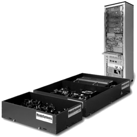 | Fig. 6. Femtosecond optical frequency comb. |
Details of the laser cooling, trapping, detecting and probing system used in this work are reported in previous works.[33– 37] We give a brief description here.
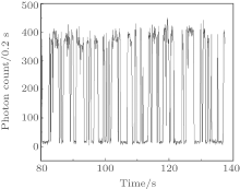
First, the trapping RF field is applied to the ring electrode, and then single ions are loaded by photo-ionization. Then, by scanning cooling laser from red detuning to resonance center, we can get the fluorescence spectrum. Typically, a 397 nm laser with approximately 10 μ W power is focused on the single ion with a spot size of about 40 μ m and 600 μ W of power, and so is the 866 nm laser, 60 μ m in size. A photomultiplier tube (PMT, 9893Q/100B, EMI) collects the weak fluorescence emitted by the laser-cooled 40Ca+ ion. The signal is amplified by a preamplifier (DC-200 MHz, Oretec) and counted by a photon counter (Stanford Research System, SR400). The experimental processes are controlled by program (LabVIEW 6.0) on a personal computer. After ions are loaded in the trap, the 397 nm laser is slowly scanned across the resonance of the 42S1/2– 42P1/2 dipole transition, while the 866 nm laser stays at the resonance to prevent decaying to the 32D3/2 state. Normally, more than one ion is trapped when just loaded. The cooling lasers are blocked several times to get a single ion, and the single trapped ion is demonstrated and detected by the quantum jump (electron shelving) technique (Fig. 7).[46]
 | Fig. 7. The quantum jump signal of a single trapped 40Ca+ ion. |
Secular motion is observed separately in the ion cloud and a single ion system, in two different ways. One is the method of RF field resonance, an additional RF voltage (DS345, Stanford Research System) of 2 V (peak to peak) is added to one of the endcaps and to one of the compensation electrodes respectively, then the frequency of the additional RF is scanned to observe a drop in the fluorescence signal; the other way is observing the secular motion sidebands of a single 40Ca+ ion’ s 42S1/2– 32D5/2 transition Zeeman profile. The secular frequencies of the trap are ω r ≈ 700 kHz and ω z ≈ 1.5 MHz.
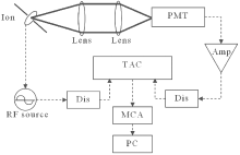
The single ion suffers excess micromotion. The amplitude of ion micromotion strongly depends on additional static electric field. Two methods of detecting ion micromotion are adopted. One relies on the alterations of atomic transition line shape; the other relies on the RF-photon correlation technique (Fig. 8).[47] A time amplitude convertor (TAC) is triggered by the output signal of the PMT, and the output signal of the RF monitor is sent to the TAC as a stop signal. The time interval is transferred to the voltage amplitude by the TAC, and the signal is sent to multi-channel analyzer (MCP) and is recorded by a computer. By observing the signal and adjusting the voltages on the compensation and endcap electrodes, the RF-photon correlation signal can be minimized and the excess micromotion is minimized in this condition.
 | Fig. 8. “ RF-Photon” correlation technique. Here, PMT: photomultiplier tube; Amp: amplitude; TAC: time amplitude convertor; Dis: discriminator; MCA: multi-channel analyzer; PC: personal computer. |
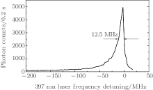
The fluorescence line shapes of single ion have been optimized by patient and repeated experiments step by step in recent years. The new results are much better than ever before: a typical counting rate of 25000 s− 1 is observed for a single cold 40Ca+ ion [Fig. 9]. The ion can be stored in the Paul trap more than one month.
 | Fig. 9. Linewidth of single-ion fluorescence signal is about 12.5 MHz and photon counts rate is up to 25000 s− 1. |
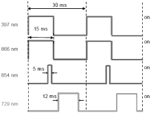
The clock transition at 729 nm is observed by the quantum jump method. In order to avoid the frequency broadening and ac Stark shift of the clock transition, the 397 nm, 866 nm, 854 nm, and 729 nm lasers are adopted as pulse sequence (Fig. 10).
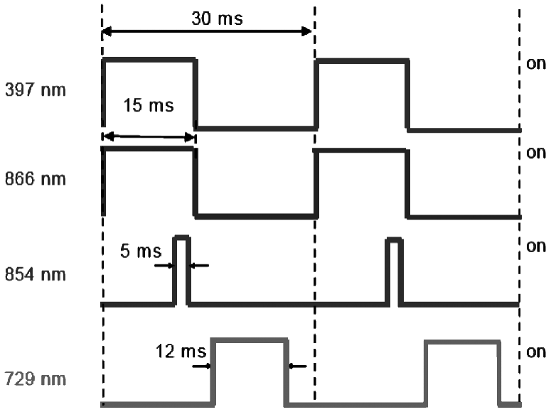 | Fig. 10. Pulse-light sequence when observing the clock transition. |
The ion is laser-cooled by the 397 nm and 866 nm lasers in the first 15 ms, and the photon counter is triggered to record the fluorescence of the ion at the same time. Then, the 854 nm laser is switched on, and irradiates the ion for 5 ms. As soon as shelved to the D5/2 state, the ion can be pumped to the P3/2 level by the 854 nm laser, and then decay to the S1/2 level. After that, a 729 nm pulse with 12 ms width is adopted, which induces a Fourier limit of a spectrum linewidth of 100 Hz (Fig. 11). In the meantime, the 397 nm, 866 nm, and 854 nm lasers are all blocked, which can reduce broadening and shift of the clock transition spectroscopy. Last, the state of the ion is checked using 397 nm and 866 nm laser pulses. If the count rate is smaller than a fixed threshold, quantum jumps take place. After the interrogation, the ion is initialized again using the 854 nm laser. The pulse sequence repeats several times.
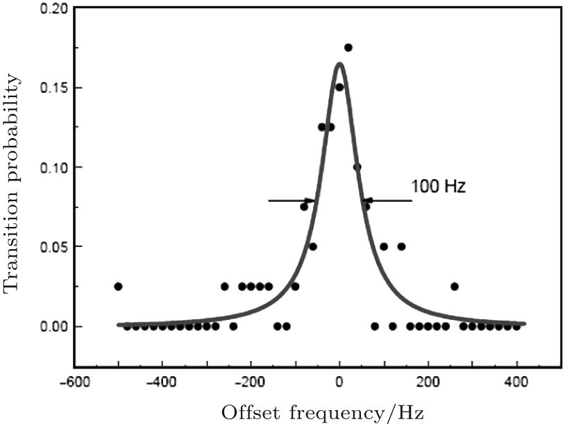 | Fig. 11. The result of scanning one Zeeman component with Δ mj = 0. |
The quantum-jumps profile of the clock resonance is adopted to investigate the quadrupole transition, which is obtained by scanning the 729 nm laser’ s frequency and recording the number of quantum jumps. When the 729 nm laser’ s frequency is close to each component’ s resonance point, more quantum jumps are detected at the same probing time or the same numbers of probe laser pulses.
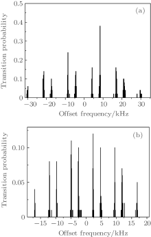
The frequency difference between the probe laser and the clock transition line center of the ion is compensated by an acoustic optical modulator (AOM). The required AOM frequencies are updated every 40 cycles of pulses, which costs about 1.5 s. By the “ 4 points locking scheme” , [48] three pairs of the Zeeman transitions (mj = ± 1/2, mj = ± 3/2, and mj = ± 5/2) are interrogated to cancel the electric quadrupole shift, [31, 32] and the offset frequency Δ f (i) between the probe laser and the transition can be obtained every 13 s (Fig. 7(a)). However, it is not easy to lock the probe laser to three pairs of the Zeeman components synchronously, since the relative intensities of the observed Zeeman components are usually different (Fig. 12(a)), and sometimes the probabilities of some of the components are very small, resulting in unstable locking of the laser to the ion. In order to get a perfect lock, the probabilities of the Zeeman components that we choose are required to be equal. In practice, the magnetic field is first compensated to be smaller than 10 nT, which means the ten components of the Zeeman profile, all together, are separated by less than 800 Hz. Then the proper angle between the direction of propagation of the laser and the direction of the B field is achieved by changing the current of the three pairs of coils. Finally, the polarization of the 729 nm laser beam is adjusted to get the best transition profile (Fig. 12(b)).
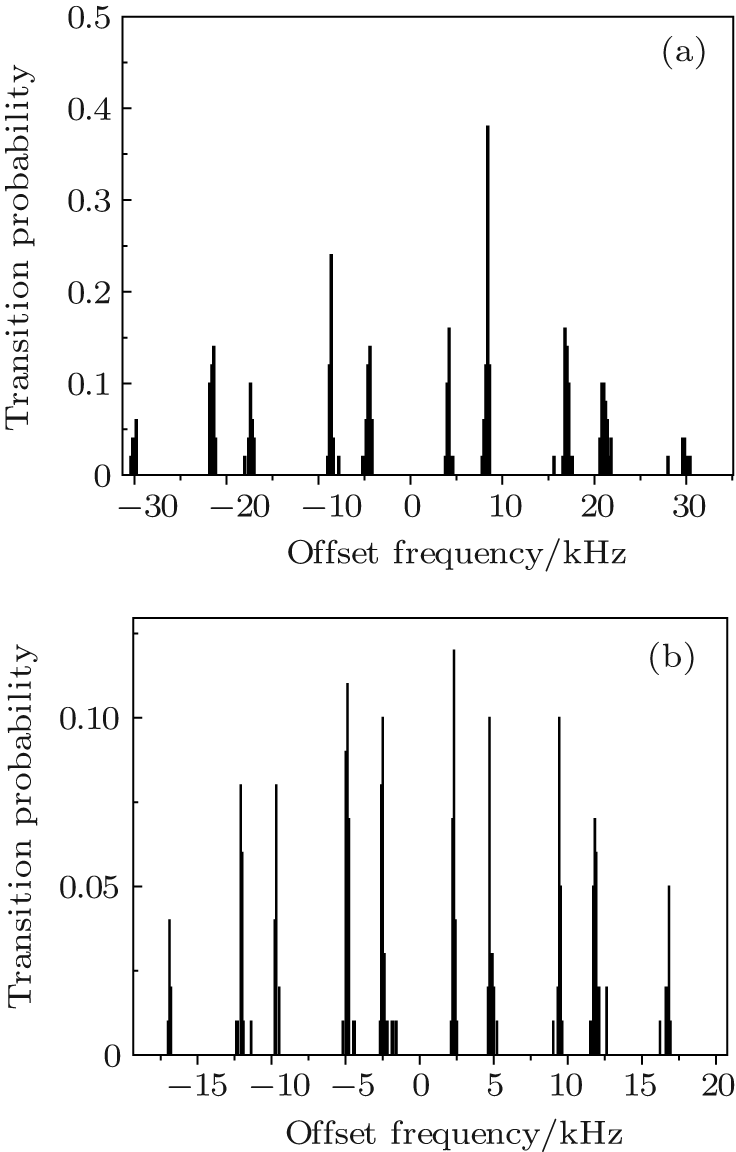 | Fig. 12. (a) Ten components of the Zeeman profile before adjusted; (b) ten components of the Zeeman profile after adjusted. |
Typically, a 854 nm laser with approximately 150 μ W power is focused on the single ion with a spot size of about 200 μ m and a typical linewidth of 10 MHz. For the 729 nm laser, we use 40 nW of power and a waist of 200 μ m.
A variety of potential sources of systematic shift are associated with the quadrupole 729 nm 4s2S1/2– 3d2D5/2 clock transition for a trapped and laser-cooled 40Ca+ ion. We shall consider the following systematic effects: the second-order Doppler effect, quadratic Stark shift (DC and AC), electric quadrupole shift, blackbody Stark shift, quadratic Zeeman shift, gravitational potential, etc. The detailed study of systematic shifts in the 40Ca+ clock transition is reported in Refs. [18] and [37].
The second-order Doppler shift is caused by the relativistic Doppler effect, due to the ion’ s motion relative to the laboratory frame, with the thermal kinetic energy and the micromotion. First of all, the micromotion should be minimized for achieving low temperature and can be measured by RF-photon correlation. After minimizing the micromotion, we can measure the second-order Doppler shift. For our ring trap, we measure the ion temperature by observing the intensity of secular sidebands. The ion temperature of 3 (3) mK is obtained by the calculation.[49] With the temperature estimated, the second Doppler shift caused by thermal kinetic energy is estimated to be − 0.004 (0.004) Hz.[47] The second Doppler shift caused by micromotion can be estimated by observing the intensity of the micromotion sidebands relative to the carrier or by observing the cross-correlation signal.[47] From the correlation signal observed, typically with a modulation amplitude ratio of 0.2 (0.1), considering that the direction of the micromotion is not well known, the shift is estimated to be − 0.02 (0.02) Hz.
Thermal secular motion and excess micromotion can push the ion out of the saddle point of the trap, which introduces a Stark shift. The Stark shift due to micromotion can be calculated from the ion temperature above; for the three pair of transitions, [47] our total averaged Stark shift due to micromotion is less than 1 mHz. According to the Stark shift due to thermal motion, for the three pairs of components as above, we can calculate from the correlation signal that the total average shift is also less than 1 mHz.[47] There is also, at the same level, a Stark shift arising from blackbody radiation. Assuming the real temperature fluctuation is 2 K at a room temperature of 293 K, the shift is 0.35 (0.02) Hz.[47]
In our experiment, during the interrogation time, all the laser beams are switched off by mechanical shutter and AOMs except for the 729 nm laser. We have measured the real efficiency of the shutter and the AOM: the attenuation of the shutter is better than 70 dB and the AOMs are better than 40 dB.
The radiations used to cool and probe the trapped ion can cause ac Stark shifts of the clock transition frequency. For the 397 nm laser, a shutter and an AOM are used to switch off the laser beam. The frequency difference between AOM on and off when doing the interrogations with the 729 nm laser is less than 10 Hz. Therefore, with an attenuation of better than 40 dB for the AOM that switches off the 397 nm radiation when the measurements are made, the shift is less than 1 mHz. For the laser at 866 nm, a shutter is used to switch off the light; the frequency difference of less than 30 Hz is measured between “ shutter always on” and “ shutter off” when doing the interrogations with the 729 nm laser. Therefore, with an attenuation of better than 70 dB for the shutter that switches off the 866 nm radiation when the measurements are made, the shift is less than 1 mHz. For the 854 nm laser beam, two individual shutters are used to block the light. The frequency difference between “ 854 nm laser off” and “ only one shutter off” when doing the interrogations with 729 nm laser is measured to be less than 20 Hz. Therefore, with an attenuation of better than 70 dB for the other shutter that switches off the 854 nm radiation when the measurements are made, the shift must be less than 1 mHz. The ac Stark shift caused by the 729 nm laser is measured by doing measurements at different probe laser intensities. From the experimental results, we obtain a linear fit slope of 0.04 (0.06) Hz/I, where I is the typical 729 nm laser intensity used for the measurements.
The linear Zeeman effect is effectively eliminated by locking to a pair of Zeeman components that are symmetric to the line center. However, there may be ac broadening of the components, and the fast changes of the dc magnetic field could cause a locking problem. As for the long term dc magnetic field drift as well as the probe laser cavity drift, we can estimate the shifts by using the servo error signal. In our case, the servo error would be 0.11 (0.03) Hz. As for the second-order Zeeman shift, it can be calculated by using the second-order perturbation theory. For our system, the average magnetic field during the measurements is 430 nT and the fluctuation of the field we measured is about 3 nT. This leads to a second Zeeman shift of less than 1 mHz, which is negligible.
There will be an electric quadrupole shift due to the presence of electric field gradients, which interacts with the electric quadrupole moment of the ion. However, by averaging the frequency of the three pairs of components, we can null the quadrupole shift.[50] According to the measured value of magnetic field drift rate, normally less than 1 nT per hour, the 6 seconds of measuring time difference can induce a shift error of less than 0.02 Hz. By averaging the difference of center frequency for different components, an error of 0.03 Hz is obtained.
There will be a gravitational shift due to gravity. A different altitude induces a different shift. We measured the altitude of our ion trap referenced to sea level by using a GPS. The measured result is 35.2 (1.0) m; thus the gravitational shift for the clock is estimated to be 1.583 (0.045) Hz.
Table 1 shows a summary of the frequency shifts considered. Systematic shifts with less than 10− 18 of the effect are not included. Taking into account all of them, we get a total fractional shift of 4.74 × 10− 15 with a fractional uncertainty of 5.0 × 10− 16 from the data obtained in May 2011 and a total fractional shift of 4.74 × 10− 15 with a fractional uncertainty of 6.5 × 10− 16 for the data obtained in June 2011.
| Table 1. Systematic frequency shifts and their uncertainties in the evaluation of the clock. Shifts and uncertainties given are in fractional frequency units (Δ ν /ν ), shifts with less than 10− 18 of effect are not included.[18] |
For the fs comb, both the repetition frequency and the offset frequency are locked to two individual synthesizers which are referenced to a 10 MHz signal provided by an active H-maser (CH1-75A) with an isolated splitter and a 60-m-long standard 50 ohm coaxial cable (RG-213). The output of the fs comb from the other PCF (with frequency of fn) is overlapped with the probe laser at 729 nm (with frequency of fc) using a PBS. The beat frequency fb = | fc – fn| between the probe laser and the n-th comb component at 729 nm is measured by two individual frequency counters referenced to the H-maser. Normally the S/N of the beat frequency is 30 dB at a resolution bandwidth of 300 kHz. However, sometimes the S/N of the beatnote drops to less than 28 dB during the measurement so that the readings are not reliable. We use two individual counters measuring the beat frequency simultaneously. If the difference of the readings of the two counters is more than 1 Hz, we believe that the measurement is not reliable and the measurement is not taken into account. The probe laser’ s frequency is measured every 1 s.
The probe laser frequency measured with the comb fc(i) could be calculated using the formula fc = nfrep ± fCEO ± fb. The integer number n could be calculated using a wavemeter with an accuracy of less than 100 MHz, and the ambiguous signs could be removed by observing the sign of the variation in the beat frequency when the repetition frequency or the carrier-envelope offset frequency is changed. Figure 8(b) shows the probe laser frequency fc(i) measured with the comb referenced to the H-maser. The observed short-term frequency noise is mainly contributed by the H-maser through the 60-m-long cable and the 20 MHz synthesizer that is used in locking the frep to the H-maser.
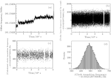
Using the two sets of the AOM offset frequency (Fig. 13(a)) and the measured probe laser frequency (Fig. 13(b)), we calculated the clock transition frequency to be ν 0(i) = fc(i) + Δ f(i) for i = 1, 2, … , imax, where imax represents the total measurements number. In the case shown in Fig. 13, the total measurement number is about 3500. Figure 13(c) shows the calculated frequency data sets of ν 0(i), which average to ν 0 = 411042129776490.7 Hz. The histogram of the ν 0(i) (Fig. 13(d)) follows a normal distribution; the standard deviation of the mean 
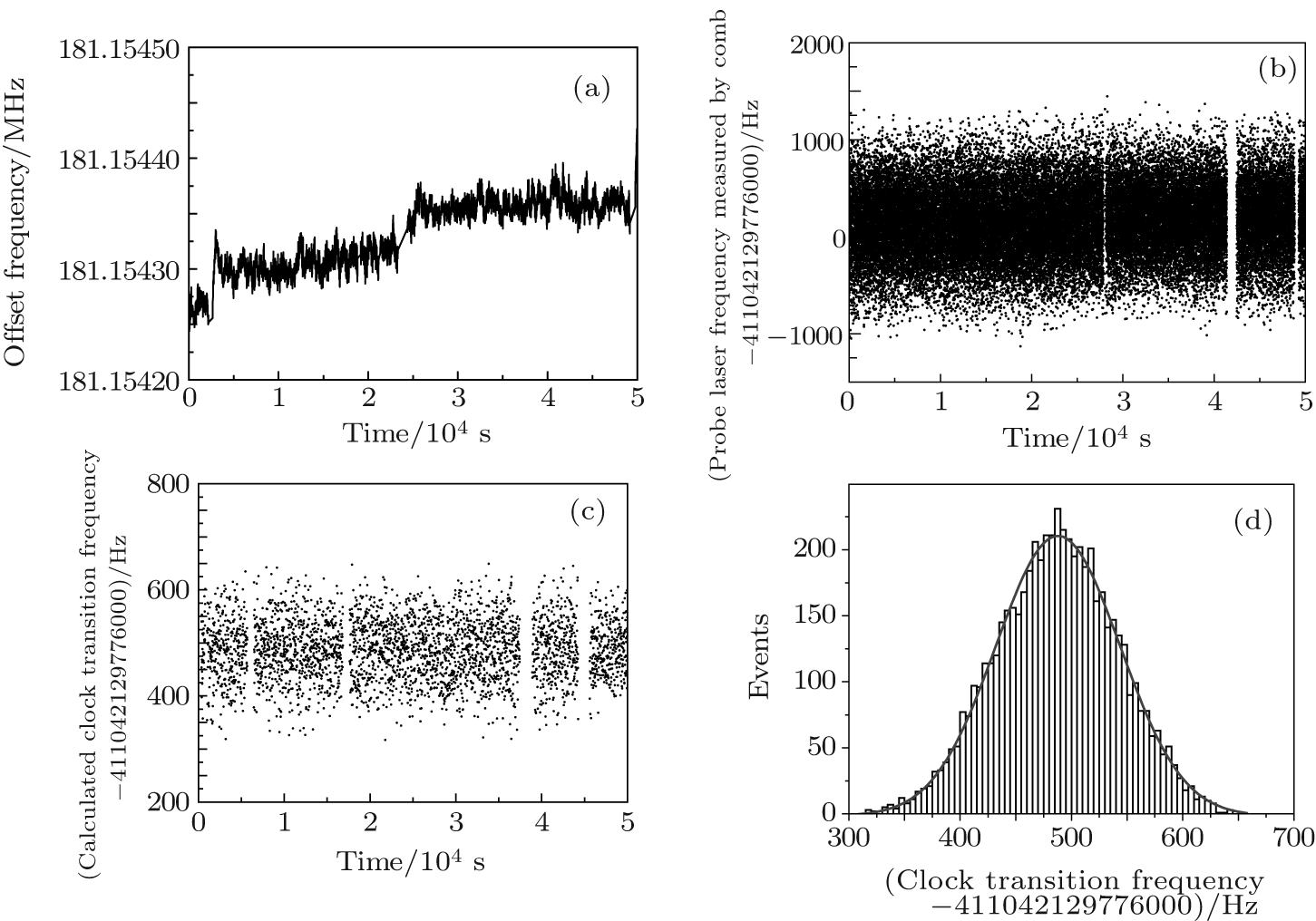 | Fig. 13. (a) Measured AOM offset frequency Δ f(i); (b) measured probe laser frequency fc(i) using the comb referenced to the H-maser; (c) frequency of the clock transition ν 0(i) calculated from Δ f(i) and fc(i); (d) histogram of the ν 0(i) with a Gaussian fitting. |
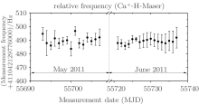
Frequency measurements were taken on 32 individual days and they were separated into two parts. One in May 2011, with 15 continuous days, and the other in June 2011, with 17 continuous days (Fig. 14). Each of the filled circles in Fig. 14 represents a mean value of ν 0(i) whose measurement is based directly on the H-maser. The error bars are given by the standard deviation of the mean
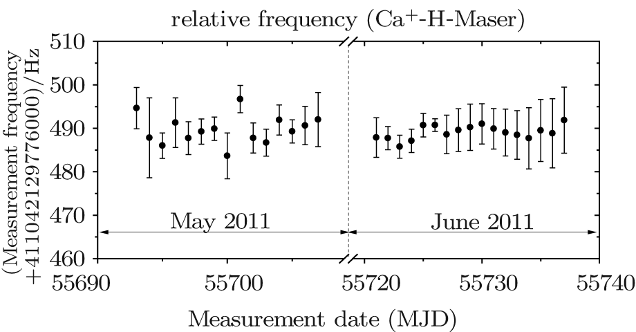 | Fig. 14. Frequency measurement of the 4s2S1/2– 3d2D5/2 transition of a laser-cooled trapped single 40Ca+ ion with reference to the H-maser. Data shown in this figure do not include systematic corrections. |
To get the final absolute frequency measurement of the clock transition, systematic shifts and the calibration of the reference must be considered and applied to the above averaged frequency. To calibrate the frequency of the H-maser, a GPS receiver with an antenna (TTS-4, PikTime Systems) is used. A detailed report on how the H-maser is calibrated using GPS can be found in Ref. [18]. Briefly, in cooperation with the National Institute of Metrology of China (NIM), the H-maser frequency was calibrated using the precise point positioning (PPP) technique, with help of GPS satellites and the frequency comparison data published on the BIPM website[51] every month. Table 2 shows the estimation for corrections to the absolute frequency of the 40Ca+ clock transition.
| Table 2. The absolute frequency measurement budget. The units of shifts and uncertainties are given in Hz.[18] |
Based upon the data listed in Table 2, we determined that the total correction for the frequency measurement shown in Fig. 8 is − 96.9 Hz for the data obtained in May 2011 and − 96.4 Hz for the data obtained in June 2011. The combined fractional uncertainty of the absolute frequency measurement is 4.6× 10− 15 for the data obtained in May 2011 and 2.6× 10− 15 for the data obtained in June 2011. The corrected absolute frequency of the 40Ca+ 4s2S1/2– 3d2D5/2 clock transition is 411 042 129 776 393.3 (1.9) Hz for the data obtained in May 2011 and 411 042 129 776 392.7 (1.1) Hz for the data obtained in June 2011. The two measurements agree with each other within their uncertainties. The unweighted mean of the above two values gives a final result of 411 042 129 776 393.0 (1.6) Hz; the final uncertainty is calculated by considering both statistical and systematical uncertainties. The obtained final result of absolute frequency measurement of the 40Ca+ 4s2S1/2– 3d2D5/2 clock transition is 411042129776393.0 (1.6) Hz, which agrees with the former measurements[17, 19] by the University of Innsbruck and the NICT.
In order to reach better performance of the 40Ca+ optical frequency standard, we have to find out which part is the limiting factor. Therefore, by the frequency comparison measurement of two 40Ca+ optical frequency standards we can achieve the performance of the individual optical frequency standard directly. The scheme of the comparison of two 40Ca+ optical frequency standards is shown in Fig. 15.[52] In our experiment, the two optical frequency standards have similar structures and share the 397 nm, 866 nm, 854 nm, and 729 nm lasers. Two AOMs (AO3 and AO4) are used to cover the difference between the clock transition frequency and the super cavity’ s resonant frequency. During the locking, although the two frequency standards share the same probe laser, the probe laser is referenced to the clock transition by feeding back to AO3 and AO4 independently to compensate for changes of the magnetic field and to address the individual Zeeman transitions. The frequency data applied to AO3 and AO4 indicate the offset values of clock transition frequencies for the two 40Ca+ optical frequency standards, whose frequency difference is reflected in the frequency difference between AO3 and AO4. To rule out the effects of the jitter of magnetic field and the drift of the probe laser frequency with time, the probe laser is locked to the clock transitions of the ions in two ion traps simultaneously and independently.
 | Fig. 15. Overview of setup for the frequency comparison of two 40Ca+ optical frequency standards. AO: acousto-optic modulator; PM: polarization maintaining; BS: polarized beam splitter. |
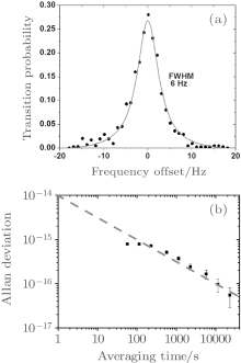
After the improvement of the performance of the clock laser, the linewidth of one Zeeman component is reduced from 100 Hz to 6 Hz (Fig. 16(a)). A preliminary optical frequency comparison experiment of the two 40Ca+ optical frequency standards is processed with the locking data of more than 3 days. A relative stability is 1× 10− 14τ − 1/2, which is shown in Fig. 16(b). The evaluation of the systematic shifts of the second 40Ca+ optical frequency standard has not been finished yet. Many systematic effects could introduce a frequency difference between the two 40Ca+ optical frequency standards. For instance, the power of the probing laser entering the ion traps is different. Therefore the final frequency difference needs to be determined with further experiments. In Fig. 16(b), the result is much better than the relative stability of the first 40Ca+ optical frequency standard versus a hydrogen maser.[18] Through this comparison of the two 40Ca+ optical frequency standards, the relative stability was found to have been improved by more than an order of magnitude.
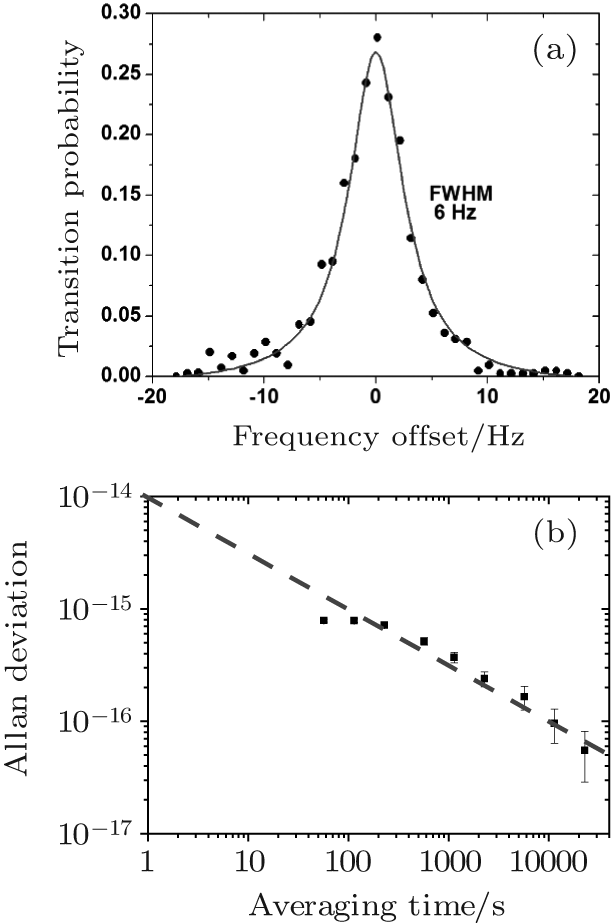 | Fig. 16. (a) 6 Hz linewidth of one component with Δ mj = 0; (b) the relative fractional stability of two independent 40Ca+ optical frequency standards. |
Singly ionized calcium is of immense research interest because of the long lifetimes of its metastable 3d2D3/2, 5/2 states (∼ 1 s), which helps to carry out many sophisticated measurements to high precision and accuracy. The long lifetime makes the electric quadrupole transition (4s2S1/2– 3d2D5/2) acquire a sub-Hz natural line width corresponding to a high quality factor (Q) value (∼ 1015) and have been considered for an optical frequency standard.
In order to accurately measure the lifetime of the 3d2D5/2 state, a high-efficiency quantum state detection method and a high precision, high synchronism measurement sequence were employed. The main measurement processes consisted of three steps in one circle period T (as Fig. 17 shown). First, the 397-nm and 866-nm lasers were turned on for 10 ms, cooling the ion down to Lamb– Dicke regime. In the first 5 ms of this laser cooling process, the 854-nm quenching laser is switched on to excite the ion from the 3d2D5/2 state to the 4p2P3/2 state to eliminate the case in which the ion stays in the 3d2D5/2 state. In the second step, the 729-nm laser is turned on 3 ms to coherently excite the 4s2S1/2– 3d2D5/2 transition. In order to eliminate the magnetic field at the position of the ion, the Hanle effect is adopted and ten Zeeman spectra are recorded with full widths < 1 kHz. In the third step, the first 3 ms is for the detection and the recording of the fluorescence of the 4p2P1/2– 4s2S1/2 transition at 397 nm. If the ion is coherently shelved to the 3d2D5/2 state, the fluorescence falls to the background level and it is regarded as a valid measurement. Then a waiting period will be followed, during which all lasers are turned off and no lights disturb the process. The whole of this step lasts Δ t, which is set to vary from 50 ms to 5000 ms. At last, in order to discriminate whether the ion decays from the 3d2D5/2 state to the ground state, a second 3-ms detection is performed. The above cycle is repeated several thousand times for every chosen Δ t in our experiment. The decay probability P is determined as the ratio of the number of quantum jumps that are counted within the second detection periods to the number counted within the first detection periods. The lifetime of the 3d2D5/2 state satisfies the exponential function P = exp(− Δ t/τ 3D5/2).
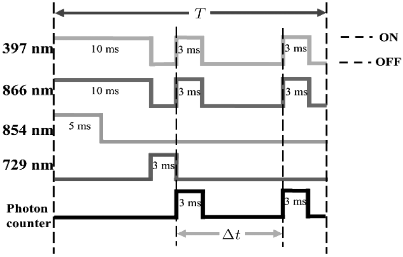 | Fig. 17. The main processes for the lifetime measurement of the 3d2D5/2 state. |
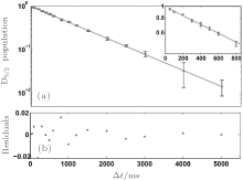
The measured result is shown in Fig. 18. Using linear regression fitting and the least squares method, the experimental data yield a lifetime τ 3D5/2 = 1171(9) ms; the residuals are shown in Fig. 18(b). And we analyzed the systematic errors of 866-nm laser intensity, collision with background gases, heating and statistical error, and the results are presented in Table 3. The final obtained value of natural lifetime is τ 3D5/2= 1174 ± 10 ms, [53] which agrees with 1168(7) ms[31] and 1168(9) ms.[32]
 | Fig. 18. Lifetime measurement result for the 3d2D5/2 state. (a) D5/2 population, (b) residuals. |
| Table 3. Error evaluation for the measurement of the lifetime of the 3d2D5/2 state. |
A magic wavelength for an atomic transition is a wavelength for which the differential ac Stark shift vanishes.[54– 57] The existence of magic wavelengths enables independent control of internal hyperfine-spin and external center-of-mass motions of atoms (including atomic ions). Precision measurements of magic wavelengths in atoms (neutral atoms and ions) are very important in studies of atomic structure.
A sketch of the experimental setup for measurement of magic wavelengths is shown in Fig. 19. The whole system is composed of two main parts: an optical clock based on the single trapped 40Ca+ and a Lm laser system for measuring the light shift of the clock transition. The Lm laser used in the experiment is frequency stabilized using a transfer cavity referenced to the 729 nm probe laser.
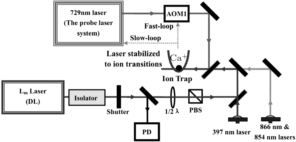 | Fig. 19. Schematic diagram of magic wavelength measurement setup. DL: diode laser; AOM: acousto-optic modulator; 1/2 λ : half wave plate; PD: photo diode; PBS: polarized beam splitter. |
The probe laser is referenced to the 40Ca+ ion clock transitions by feeding back to the frequency of the acousto– optic modulator (AOM1) to compensate for changes of the magnetic field and address of individual Zeeman transitions. In the experiment, the pulse sequences of 397 nm, 866 nm, 854 nm, and 729 nm lasers are similar to those used in the 40Ca+ ion optical frequency standard.[18, 37] The pulse sequence of the Lm laser is introduced to measure the light shift. The Lm laser is off during the Doppler cooling period, and is on and off alternately during probing stage to measure the light shift. The frequency values of AOM1 are recorded automatically every cycle by a PC, and the light shift caused by the Lm laser beam can be measured by calculating the difference of two cycles with the Lm laser on and off. Ac Stark shifts within 0.2 nm around the magic wave-length λ mj were studied. Six randomly fixed wavelengths of the Lm laser were chosen, and the ac Stark shift was measured at each wavelength by switching on/off the Lm laser. The six measured points are fitted linearly to obtained the magic wavelength.
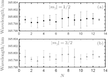
Two magic wavelengths for the 40Ca+ clock-transition were measured simultaneously. Here 10 instances of λ | mj| = 1/2, λ | mj| = 3/2 measurements and the trimmed means yield λ | mj| = 1/2 = 395.7992(2) nm and λ | mj| = 3/2 = 395.7990(2) nm, as presented in Fig. 20, and mj is the magnetic quantum number of the 3D5/2 state. The difference in value between λ | mj| = 1/2 and λ | mj| = 3/2 is 0.0002(6) nm, which agrees with the previous theoretical calculation.[58]
 | Fig. 20. (a) Ten measurements of λ | mj| = 1/2 (black squares). (b) Ten measurements of λ | mj| = 3/2 (blue triangles) under the same conditions with λ | mj| = 1/2. The errors indicated are the statistical errors of the measurements. The solid circle spots and the solid purple triangle indicate the weighted mean, and the errors are obtained from the weighted average of statistical errors. |
To get the final magic wavelength measurement of the Lm laser, systematic shifts have been considered. These shifts include the broad spectral component, the light polarization, the second-order Doppler shift, the calibration of the wavemeter, etc. An error budget is given in Table 4. In the end, two magic wavelengths, 395.7992(7) nm and 395.7990(7) nm in the spin– orbit energy gap of the 4p state were identified.[59]
| Table 4. Magic wavelength measurement uncertainty budget. |
Systematic frequency measurements were made of the 40Ca+ clock transition at 10− 15 level with a laser-cooled single ion in a miniature Paul trap. We used GPS to calibrate the H-maser and we performed the measurements for a long averaging time (32 days with more than 2 million seconds of measurements) to approach a measurement accuracy level of 10− 15. With the GPS PPP technique, we achieved a frequency transfer uncertainty of about 1 × 10− 14 with an averaging time of one day. The total systematic error for the clock transition frequency is better than 6.5 × 10− 16. To achieve a smaller uncertainty, we will need to use a more stable reference to reduce the statistical error. In fact, we find that the uncertainty of the linear Zeeman shift is limiting the final systematic uncertainty. The uncertainty due to the linear Zeeman effects is mainly caused by the fluctuation of the magnetic field, which can be measured by calculating the variance of the Zeeman splitting of the Zeeman transitions. According to the variance of the Zeeman splitting, the uncertainty is calculated from statistics. We processed the preliminary comparison of two 40Ca+ optical frequency standards and the relative stability 1 × 10− 14τ − 1/2 was found.
To reduce the systematic uncertainties in the future, one has to increase the stability of the magnetic field. We also want to do a comparison experiment between WIPM and NICT or University of Innsbruck by the GPS. A Cs fountain may be introduced to do a new round of measurement to make the results even better possibly approaching the 10− 16 level.
We observed the lifetime of the 3d2D5/2 state in 40Ca+ by recording the quantum jumps of a single ion trapped in a miniature ring Paul trap. High precision multi-channel pulse sequences are adopted with an accuracy of the microsecond level. We obtain the value of natural lifetime of the 3d2D5/2 state = 1174± 10 ms, which agrees with two previous measurements[31, 32] but differs from other reported values. Although the single 40Ca+ ion is laser-cooled to the Lamb– Dicke regime by us and in the measurement schemes of Refs. [31] and [32], ours is a ring Paul trap while the others used the linear Paul trap. Nevertheless, improvement in the accuracy of our measurement is still possible by collecting more quantum jumps in a better vacuum condition.
Experimental determinations of the magic wavelengths of the 40Ca+ clock transition were processed with uncertainty better than 0.001 nm, which is realized for the first time in the ion optical clock systems. The specific values are λ | mj| = 1/2= 395.7992(7) nm and λ | mj| = 3/2 = 395.7990(7) nm. The uncertainty from broadband light and statistical error were the largest contributors to the total uncertainty. A cavity for mode selection to the Lm laser can be used to reduce the uncertainty from broadband light and the uncertainty from statistical error can be improved by improving power stabilization. An order of magnitude improvement in the precision of these measured magic wavelengths is achievable.
We acknowledge Gui-Long Huang, Xue-Ren Huang, Hua-Lin Shu, Bin Guo, Hao-Quan Fan, Qu Liu, Wan-Cheng Qu, Bao-Quan Ou and Jian Cao for the early works, thank Zhi-Yi Wei, Kun Liang, Tian-Chu Li, Jim Mitroy, Bijaya Sahoo, Ying Li Ting-Yun Shi, Cheng-Bin Li, Li-Yan Tang, and Yong-Bo Tang for cooperation, and Jun Ye, Kensuke Matsubara, Patrick Gill, James Bergquist, Long-Sheng Ma, Yi-Qiu Wang, Yu-Zhu Wang, Chao-Hui Ye, Jun Luo, Ming-Sheng Zhan, Jia-Ming Li, Zong-Chao Yanand Chao-Hong Lee for their fruitful discussion and suggestions.
| 1 |
|
| 2 |
|
| 3 |
|
| 4 |
|
| 5 |
|
| 6 |
|
| 7 |
|
| 8 |
|
| 9 |
|
| 10 |
|
| 11 |
|
| 12 |
|
| 13 |
|
| 14 |
|
| 15 |
|
| 16 |
|
| 17 |
|
| 18 |
|
| 19 |
|
| 20 |
|
| 21 |
|
| 22 |
|
| 23 |
|
| 24 |
|
| 25 |
|
| 26 |
|
| 27 |
|
| 28 |
|
| 29 |
|
| 30 |
|
| 31 |
|
| 32 |
|
| 33 |
|
| 34 |
|
| 35 |
|
| 36 |
|
| 37 |
|
| 38 |
|
| 39 |
|
| 40 |
|
| 41 |
|
| 42 |
|
| 43 |
|
| 44 |
|
| 45 |
|
| 46 |
|
| 47 |
|
| 48 |
|
| 49 |
|
| 50 |
|
| 51 |
|
| 52 |
|
| 53 |
|
| 54 |
|
| 55 |
|
| 56 |
|
| 57 |
|
| 58 |
|
| 59 |
|