Double optomechanical transparency with direct mechanical interaction*
[Li Ling-Chao, Shi Rao, Xu Jun, Hu Xiang-Ming† ]
]
]
|
|


†Corresponding author. E-mail: xmhu@phy.ccnu.edu.cn
*Project supported by the National Natural Science Foundation of China (Grant Nos. 61178021, 11474118, and 11204099) and the National Basic Research Program of China (Grant No. 2012CB921604).
We present a mechanism for double transparency in an optomechanical system. This mechanism is based on the coupling of a moving cavity mirror to a second mechanical oscillator. Due to the purely mechanical coupling and the radiation pressure, three pathways are established for excitations of the probe photons into the cavity photons. Destructive interference occurs at two different frequencies, leading to double transparency to the probe field. It is the coupling strength between the mechanical oscillators that determines the locations of the transparency windows. Moreover, the normal splitting appears for the generated Stokes field and the four-wave mixing process is inhibited on resonance.
Electromagnetically induced transparency (EIT) is a quantum interference effect observed in atomic or molecular systems, in which the response of the atoms or molecules to the probe field is controlled by a coupling field.[1– 3] It has been demonstrated that EIT has a variety of potential applications, such as giant nonlinear effects[4– 8] and slow light.[9– 12] As a physical mechanism for EIT, quantum interference occurs between two pathways for the probe absorption when the coupling field is coupled to a cascaded clock transition in a Λ configuration.
Recently, it was found that an optomechanical system displays a similar effect. A radiation pressure force induces the optomechanical coupling, [13] which creates two pathways for the excitations of the probe field into the cavity field. Once the interference occurs between these two pathways, the optomechanically induced transparency (OMIT) appears.[14– 24] Agarwal et al.[14] analyzed the absorptive and dispersive responses of an optomechanical system to the probe field and showed why EIT emerges in the optomechanical system. Weis et al.[15] reported an experimental realization by tuning the coupling field to a sideband transition of an optomechanical system.
In this paper, we show that it is possible to achieve double transparency by employing a purely mechanical coupling in an optomechanical system. Earlier, the double transparency was demonstrated for a multilevel atomic system.[25– 31] When the coherent coupling establishes three pathways for the absorption of the probe field, the destructive interference can be obtained at two different frequencies, which corresponds to the double transparency. Most recently, several schemes have been proposed to achieve double OMIT.[32– 35] Among them are systems with two mechanical oscillators coupled to a common cavity field.[32, 33] However, these systems are subjected to a special limit. The two oscillators have to have different frequencies. Once the frequencies are the same, the optomechanical transitions become degenerate and the transparency is only possible at one frequency.
In order to overcome this limit, we consider the effect of the purely mechanical interaction on the optomechanical response. A mechanical oscillator is coupled to the moving mirror but not to the cavity field, and the mechanical interaction occurs between the cavity mirror and the extra oscillator. The two involved oscillators can have the same frequency. Such a combination of mechanical interaction with the optomechanical coupling will create three pathways for the excitations of the probe field into the cavity field. Destructive interference occurs at two different locations. The remarkable feature of the present scheme is the controllable locations of the transparency windows, which are determined by the coupling strength of the two mechanical oscillators. When we increase the internal mechanical coupling strength between the two oscillators, the locations of the two EIT windows move further away from each other. Equivalently, in terms of the collective modes, the two oscillators in our model are transformed into two effective ones, whose frequencies depend on the oscillator coupling strength. The two effective oscillators no longer interact with each other, but they are both coupled to the cavity field. The transparency windows appear at the coupling strength dependent frequencies.
In addition, as the coupling power increases, the two EIT windows are broadened. The normal splitting also appears in the generated Stokes field and the inhibition of the four-wave process can be observed on resonance. The above optomechanical device has been investigated in a recent experiment by Lin et al., [16] who have studied coherent mechanical mode mixing in the double-disk cavity. Therefore the present scheme is within the experimentally accessible technology.
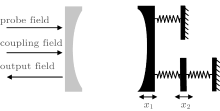
We consider the optomechanical system shown in Fig. 1. The right mirror is perfectly reflecting and oscillating, and its displacement from its balance position is denoted as x1. The left mirror is fixed and partially transmitting. Through the left mirror, a strong input coupling laser field of frequency ω c drives the cavity field, which gives rise to the radiation pressure on the right mirror. At the same time, a weak probe field of frequency ω p is sent into the cavity. In the present work, we would like to consider the mechanical effects on the probe absorption in such an optomechanical system. To do this, we assume that the moving end mirror is linked to a second mechanical oscillator (its displacement from its balance position is denoted as x2) through a spring. In the present optomechanical system, the cavity field is coupled only to the first oscillator but not to the second oscillator. Such a system was studied by Lin et al., [16] who demonstrated the optical control of mechanical motion. Here we focus on the mechanical effects on the probe field absorption. The mechanical oscillators can be described by the Hamiltonian
where ω j is the frequency (although we will consider the same frequency, we keep the subscripts for discriminating different oscillators), mj is the effective mass, and pj is the moment of the j oscillator, j = 1, 2. The last term describes the internal interaction between the moving mirror and an auxiliary oscillator, and χ is the coupling coefficient between the two oscillators.
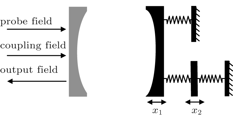 | Fig. 1. Schematic diagram of the optomechanical system studied in the present paper. A strong coupling field of frequency ω c and a weak probe field of frequency ω p are injected into the cavity through the fixed partially transmitting left mirror. The right moving cavity mirror (denoted by x1) and the second oscillator (denoted by x2) coherently couple with each other. Only the moving cavity mirror interacts with the cavity field. |
As usual, we consider the case for which the frequency of the moving mirror is much smaller than the cavity free spectral range c/2L (c is the speed of light in vacuum, and L is the cavity length in the absence of the intracavity field). Thus we can neglect the photon scattering into the other modes and restrict the model to the case of a single-cavity mode.[36, 37] In a frame rotating at the driving frequency ω c, the Hamiltonian describing the interaction of the cavity field with the oscillator and the coupling and the probe fields can be written as

The first term is the free energy of the cavity field, the second term describes the nonlinear optomechanical interaction between the cavity field and the moving mirror, and g = ω 0/L is the optomechanical coupling strength, with ω 0 being the resonance frequency of the cavity field. The last two terms describe the interactions of the cavity field with the coupling and the probe fields, respectively. The parameters 
We are interested in the mean response of the system to the probe field. We first derive the equations of motion from the Hamiltonian H1+ H2 as follows:

where γ 1, 2 are the damping rates of the two oscillators. The coupling field provides a steady-state solution (as, x1s, x2s) of the system, while the probe field causes a perturbation to the steady state. We can use the perturbation method to deal with the response of the probe field. In the presence of modulation terms like e± iδ t and due to the weakness of ɛ p, we expand the total solution of the intra-cavity field and the mechanical displacements to the first-order sidebands

where the zero-order solutions (with subscript “ s” ) are obtained from Eq. (3) as
with Δ = ω 0 − ω c − gx1s. As usual, we tune the coupling field such that the condition Δ = ω m is met. We see from Eq. (5) that the displacement x1s depends on the number of cavity photons, equivalently, on the power of the coupling field. In a general case, the present system can exhibit bistability. However, here we focus on the case in which the oscillator frequencies are equal ω 1 = ω 2 = ω m and the displacement x1s has one solution. This is guaranteed by Pc < 72 mW for the experimentally realizable parameters:[17]m1 = m2 = 12 ng, ω m = 2π × 10 MHz, κ = 2π × 0.4 MHz, L = 6 mm, λ = 2π c /ω c = 1064 nm, γ 1 = γ 2 = 200 Hz, χ = 103 J/m2.
The equations of motion for the first-order perturbations are derived as

where 
Using the input– output relation, [38] we obtain

We expand the output field to the first-order sidebands

where ɛ out0, ɛ out− , and ɛ out+ are the components of the output field oscillating at frequencies ω c, ω p = ω c+ δ , and 2ω c− ω p = ω c − δ , respectively. Here ɛ out+ represents a Stokes field, and is generated via the nonlinear four-wave mixing process. Substituting Eq. (8) into Eq. (7), we find that the components of the output field at the probe frequency and the Stokes frequency are, respectively,

As a comparison, in the absence of the coupling field (Pc = 0), the components of the output field at the probe frequency and the Stokes frequency are given, respectively, by

Here we focus on the case of Pc ≠ 0. In what follows we consider the quantity

According to the theory of the absorption and dispersion, it is clear that the real and the imaginary parts, Re(μ ) and Im(μ ), represent the absorption and the dispersion, respectively. These quantities can be measured by the homodyne technique.[39]
In this section, we present our numerical results in the following three aspects by using the parameters given in the above section and by plotting the dimensionless quantity Re(μ ) as a function of the normalized detuning δ /ω m (i.e., the probe field detuning δ = ω p − ω c in the unit of the oscillator frequency ω m).
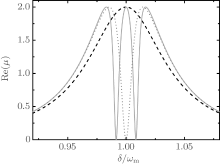
First, in Fig. 2, we compare the quadrature of the output field around ω = ω c + ω m for three different cases. (i) Pc = 0 and χ = 0. In this case, there is neither an optomechanical coupling nor a purely mechanical coupling. We see that Re(μ ) has a standard Lorentzian peak (black dashed curve). (ii) Pc ≠ 0 and χ = 0. This corresponds to the case in which there is an optomechanical interaction but no purely mechanical coupling. For this case, Re(μ ) displays a narrow EIT-like dip at the line center (blue dotted curve). The system becomes transparent for the probe field. (iii) Pc ≠ 0 and χ ≠ 0. The optomechaical coupling and the purely mechanical coupling combine to take effect (red solid curve). Here we take the coupling field power 20 mW and the mechanical coupling coefficient 800 J/m2. The system exhibits two symmetric narrow dips and an absorption peak in the line center. The purely mechanical coupling induces two EIT windows around the frequency ω = ω c + ω m
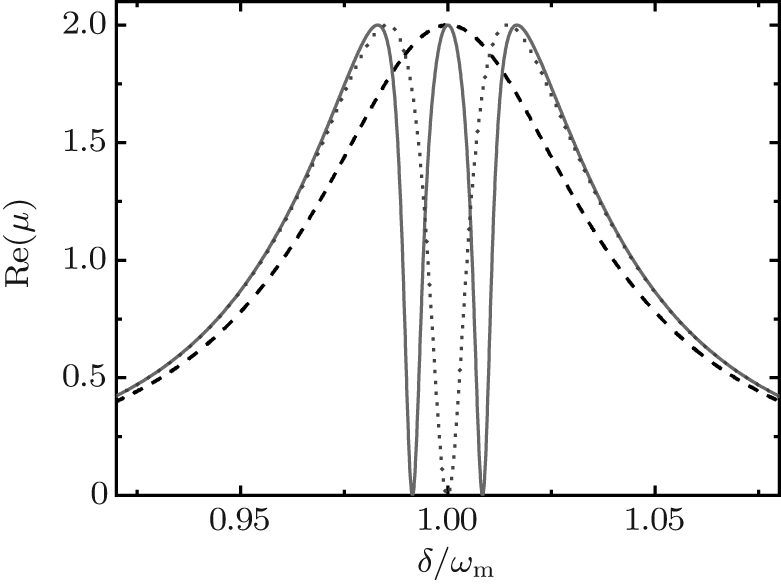 | Fig. 2. The quadrature of the output field around ω = ω c+ ω m versus the normalized probe detuning δ /ω m. The parameters are chosen as Pc = 0 mW and χ = 0 J/m2 (black-dashed), Pc = 20 mW and χ = 0 J/m2 (blue-dotted), and Pc = 20 mW and χ = 800 J/m2 (red-solid), respectively. |
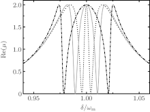
Second, we show in Fig. 3 the dependence of the probe absorption around ω = ω c + ω m on the strength of the mechanical coupling. We compare the probe absorption for three different coupling coefficients χ = 400 J/m2 (black-solid), 1000 J/m2 (red-dotted), and 2000 J/m2 (black-dot-dashed). The mechanical coupling strength is chosen as Pc = 20 mW. It is obvious that the locations of the EIT windows are remarkably dependent on the mechanical coupling strength χ . As χ increases, the two EIT windows are shifted far away from each other.
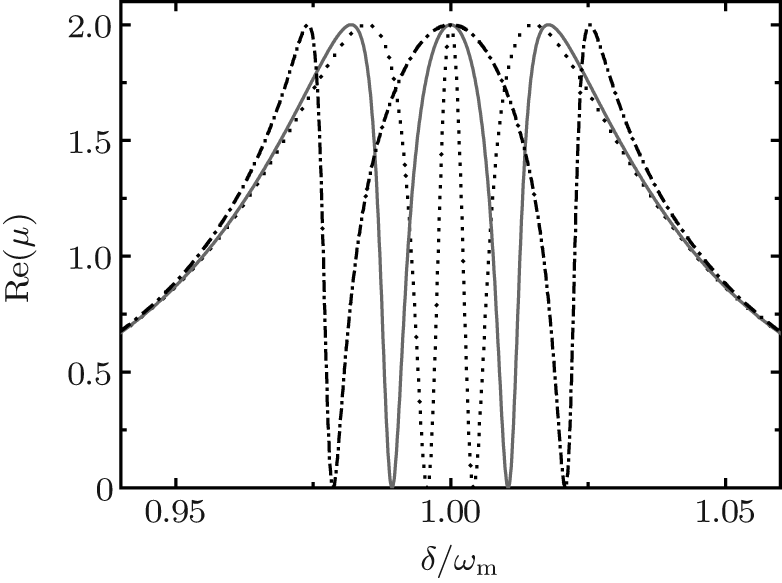 | Fig. 3. Dependence of the quadrature of the output field around ω = ω c+ ω m on the mechanical coupling strength for Pc = 20 mW. The black-dotted, red-solid, black-dot-dashed curves correspond to χ = 400 J/m2, 1000 J/m2, 2000 J/m2, respectively. |
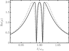
Third, the transparency windows are broadened as the mechanical coupling strength or the coupling field power increases. It can be found from Fig. 3 that the transparency windows broaden slightly as we increase the mechanical coupling strength χ . Figure 4 shows clearly that an increase in the coupling field power Pc widens the EIT windows while the locations of the two EIT windows remain unchanged.
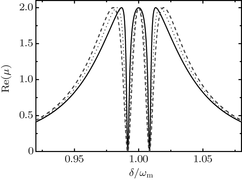 | Fig. 4. Dependence of the quadrature of the output field around ω = ω c+ ω m on the power of the coupling field for χ = 800 J/m2. The black-solid, red-dotted, blue-dashed curves correspond to Pc = 10 mW, 20 mW, 30 mW, respectively. |
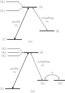
In order to understand the physical mechanism behind the above results, we use the dressed-state picture to describe the excitations of the probe field into the cavity. Let us take three adjacent states | 1〉 = | np, nb〉 , | 2〉 = | np, nb+ 1〉 , and | 3〉 = | np+ 1, nb〉 , as shown in Fig. 5(a). The | 1〉 → | 3〉 transition describes the excitation of the probe field into the cavity field. The excitation is controlled by the resonant clock transition | 2〉 → | 3〉 due to the coupling field.[14, 15] The clock transition induced by the coupling field causes the Autler– Townes splitting of the level | 3〉 into a doublet | 31, 2〉 . The original transition | 1〉 → | 3〉 is split into two pathways | 1〉 → | 31, 2〉 , which have different but close frequencies. Once a destructive interference occurs at the center frequency, the optomechanical system becomes transparent to the probe field. Essentially, this mechanism is the same as that for EIT in the three-level Λ atomic system.[1– 3] Our numerical results are explained correspondingly from the following three aspects.
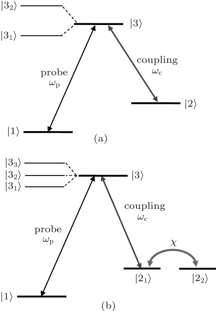 | Fig. 5. Dressed state mechanism for the probe absorption. (a) Three-level structure and the transitions for an optomechanical system with one moving mirror. (b) Level structure and transitions for two mechanical oscillators of the same frequency, one of which is the moving mirror and is coupled to the cavity field, while the other is a mechanical oscillator linked to the moving mirror but not coupled directly to the cavity field. |
First, the present double transparency is due to the quantum interference between three pathways, which are based on the interaction between the two mechanical oscillators, as shown in Fig. 5(b). We have two optomechanical states | 21〉 = | np, nb1+ 1〉 and | 22〉 = | np, nb2+ 1〉 for the coherent control. These two states are coupled to each other via the direct mechanical interaction. Only the former state | 21〉 is coupled to the coupling field, the latter state | 22〉 is not. In this way, we have a cascade of optomechanical and purely mechanical interactions. Such interlinked interactions lead to a triplet splitting of the state | 3〉 into a triplet | 31, 2, 3〉 . Correspondingly, the original transition | 1〉 → | 3〉 is split into three pathways | 1〉 → | 31, 2, 3〉 . In this case, the destructive interference can occur at two different frequencies, which locate at two sides symmetrically. Thus we have three excitation pathways and destructive interference at two different frequencies. This explains the double OMIT.
Second, we study how the locations of transparency depend on the parameters. The result can be given by using the collective oscillators as follows, one is the average coordinates (P1, Q1) and the other is the relative coordinate (P2, Q2):
With these new coordinates, we can rewrite Eqs. (1) and (2) of the system Hamiltonian (with the same frequencies ω 1 = ω 2 = ω m and the same masses m1 = m2 = m) as

where 

Third, the broadening of the transparency windows is due to the saturation effects of the mechanical coupling strength χ and/or the coupling field power Pc. When we increase the mechanical coupling strength χ or the coupling field power Pc, the space between the adjacent two levels of the triplet | 31, 2, 3〉 in Fig. 5 becomes large. This leads to a larger range for the destructive interference. Therefore, as the mechanical coupling strength χ (Fig. 3) or the coupling field power increases (Fig. 4), the transparency windows become slightly wide.
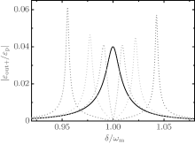
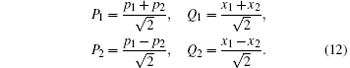
After analyzing the physical mechanism for OMIT, we now present the output Stokes spectrum of the probe field. As we know, there is no Stokes field if there is no optomechanical interaction. When the power of the coupling field is not too high, in the absence of the coupling oscillator x2, the optomechanical coupling leads to the spectral peak at the line center ω = ω c− ω m. However, once the purely mechanical coupling is introduced, the Stokes spectrum exhibits normal mode splitting and the four-wave mixing effect is completely suppressed on resonance, as shown in Fig. 6. Moreover, with the increase of the mechanical coupling strength of the two oscillators, the two peaks are pushed further away from each other, and the peak heights are increased.
 | Fig. 6. The amplitude for the Stokes field | ɛ out+ /ɛ p| around ω = ω c− ω m versus the normalized probe detuning δ /ω m for Pc = 20 mW. The black-solid, red-dashed, green-dashed, blue-dashed curves correspond to χ = 0 J/m2, 800 J/m2, 2000 J/m2, 4000 J/m2, respectively. |
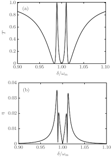
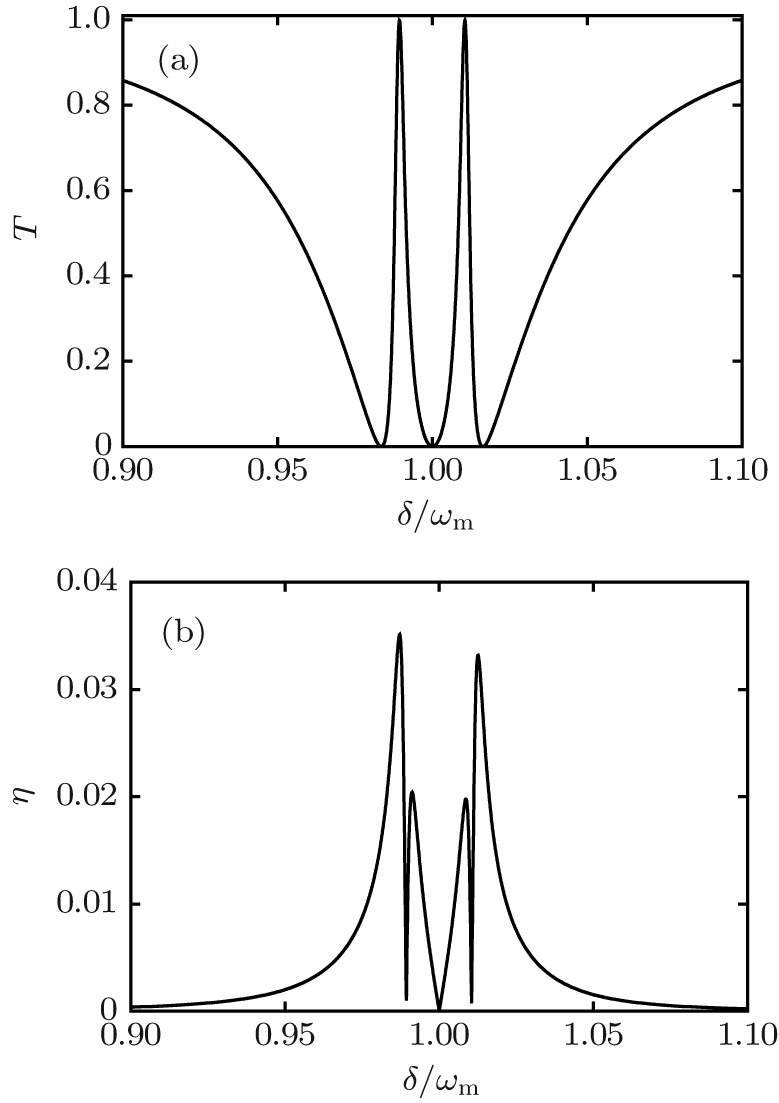 | Fig. 7. (a) The transmission coefficient T around ω = ω c+ ω m and (b) the second-order sideband efficiency η around ω = ω c+ 2ω m versus the normalized probe detuning δ /ω m for Pc = 30 mW and χ = 1000 J/m2. |
It is interesting to compare the present scheme with the previous ones. Among them is that proposed by Huang.[33] When the two moving mirrors of different frequencies are simultaneously coupled to the cavity field, [32, 33] we have two different optomechanical states | 21〉 = | np, nb1+ 1〉 and | 22〉 = | np, nb2+ 1〉 for the coherent control. The coherent transitions | 21, 2〉 → | 3〉 split the state | 3〉 into a triplet of different but close frequencies. However, once these two oscillators have the same frequency, the middle state of the triplet decouples from the probe field. Only the other two are left for the excitations. In this case, only two excitation pathways interfere with each other and the transparency is possible at a single frequency. This difficulty is overcome, as in our scheme, by coupling one oscillator to the cavity field and letting the second oscillator decouple from the cavity field. The present scheme is realizable based on the recent experiment of Lin et al.[16]
So far, our analysis and comparison have been confined to the first-order sideband. In fact, the higher order sidebands exist, although they are negligibly weak. Xiong et al.[21] considered the second-order sidebands for a single transparency window in an optomechanical system. Here we show the second order sidebands for the double transparency optomechanical system. Following the same technique above and including the second-order sideband terms e± 2iδ t in the ansatz (4), we can examine the second-order sidebands. Using the second-order expansion for the output field 

We have studied the effects of a cascade of optomechanical and purely mechanical interactions on the probe absorption and have shown the double transparency windows. In the optomechanical system considered, the cavity field interacts with the moving cavity mirror, and the latter is linked to a second mechanical oscillator via a spring, but no direct interaction exists between the cavity field and the second oscillator. The cascade interactions split the original excitation transition into three, and the destructive interference between them occurs at two different frequencies. As a result, the absorption of the probe field is canceled at these two frequencies and double transparency occurs. The characteristic feature is that the the two transparency windows are determined by the mechanical coupling strength. This suggests a different way to manipulate the locations of the double transparency windows. In addition, we have shown the normal splitting of the generated Stokes field and the inhibition of four-wave mixing on resonance.
| 1 |
|
| 2 |
|
| 3 |
|
| 4 |
|
| 5 |
|
| 6 |
|
| 7 |
|
| 8 |
|
| 9 |
|
| 10 |
|
| 11 |
|
| 12 |
|
| 13 |
|
| 14 |
|
| 15 |
|
| 16 |
|
| 17 |
|
| 18 |
|
| 19 |
|
| 20 |
|
| 21 |
|
| 22 |
|
| 23 |
|
| 24 |
|
| 25 |
|
| 26 |
|
| 27 |
|
| 28 |
|
| 29 |
|
| 30 |
|
| 31 |
|
| 32 |
|
| 33 |
|
| 34 |
|
| 35 |
|
| 36 |
|
| 37 |
|
| 38 |
|
| 39 |
|