


A novel phase-sensitive scanning near-field optical microscope*
Cite this Article
Wu Xiao-Yu, Lin Sun, Tan Qiao-Feng, Wang Jia. A novel phase-sensitive scanning near-field optical microscope* . Chinese Physics B, 2015, 24(5): 054204 
Permissions
A novel phase-sensitive scanning near-field optical microscope*
†Corresponding author. E-mail: tanqf@mail.tsinghua.edu.cn
*Project supported by the National Natural Science Foundation of China (Grant Nos. 61177089, 61227014, and 60978047).
Abstract
Phase is one of the most important parameters of electromagnetic waves. It is the phase distribution that determines the propagation, reflection, refraction, focusing, divergence, and coupling features of light, and further affects the intensity distribution. In recent years, the designs of surface plasmon polariton (SPP) devices have mostly been based on the phase modulation and manipulation. Here we demonstrate a phase sensitive multi-parameter heterodyne scanning near-field optical microscope (SNOM) with an aperture probe in the visible range, with which the near field optical phase and amplitude distributions can be simultaneously obtained. A novel architecture combining a spatial optical path and a fiber optical path is employed for stability and flexibility. Two kinds of typical nano-photonic devices are tested with the system. With the phase-sensitive SNOM, the phase and amplitude distributions of any nano-optical field and localized field generated with any SPP nano-structures and irregular phase modulation surfaces can be investigated. The phase distribution and the interference pattern will help us to gain a better understanding of how light interacts with SPP structures and how SPP waves generate, localize, convert, and propagate on an SPP surface. This will be a significant guidance on SPP nano-structure design and optimization.
Keyword:
42.30.Rx; 52.25.–b; 07.79.Fc; 06.30.Ka; phase detection; scanning near-field optical microscope (SNOM); heterodyne interferometry; surface plasmon polariton (SPP) devices
1. Introduction
Since the invention of the scanning near-field optical microscope (SNOM), it has been widely used for studying the optical properties of samples in the near field.[1, 2] With a classic SNOM system, the topography and the intensity distribution can be obtained simultaneously, while the optical phase information is lost during probing. The optical phase is a fundamental parameter for electromagnetic waves and most surface plasmon polariton (SPP) devices are designed based on phase matching. The phase distribution helps to reveal the interactions between the optical field and nano-structures, such as integrated optics, nano-photonics, cavities, resonators, etc. Hillenbrand and Neaspec Gmbh have successfully developed a near filed optical phase measurement system based on the scattering SNOM (s-SNOM) with an apertureless AFM tip combined with the heterodyne interferometry and they have obtained many beautiful phase mapping results.[3– 5] Measuring with an apertureless tip has the advantage of high spatial resolution. It is good at mapping the localized fields on the surfaces of tiny structures, especially for charge distribution and Fano-resonance, but weak for mapping the phase distribution of a propagating field at an arbitrary position in space. Since the apertureless tip has an enhancement in the Z direction, [6] it is not good at measuring the in-plane (X– Y) field distributions of SPP devices. The Herzig group also achieved phase and amplitude mapping with aperture fiber probes. Their system worked at infrared wavelengths based on optical fibers.[7– 10] Nesci studied the phase singularities of an optical propagating field with a phase detection system, [11] which was based on the sample scanning mode. It can realize phase mapping in arbitrary position in space, but it is not suitable for investigating the effect of various parameters of SPPs because scanning the sample may change the illumination condition and affect the excitation of SPPs. Several groups from Netherland and France also achieved phase mapping with different methods.[12, 13] Currently. there are still few publications on SPP’ s phase measurement.
In this paper, we demonstrate a system working at the visible spectrum with optimized optical path architecture and flexible illumination configuration, which can synchronously map topography, phase, and amplitude distributions. Both the localized field and the propagating field can be measured by this system. Compared with infrared, the visible light theoretically provides a higher resolution. The flexible illumination platform supports various SPP excitation requirements. The fiber path is more stable and has the advantage of being disturbance proof for signal transmission, while the spatial light path shows a more flexible adjustment according to complex illumination requirements.
2. Principle of phase retrieved system
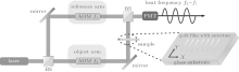
The optical frequency is as high as 1014 Hz in the visible range, photo detectors cannot follow the instantaneous oscillation of the electric field. The output of a detector is the result of the energy integration.[14] This measurement is incomplete because an electromagnetic field has not only an intensity but also a phase, which is systematically lost in such a measurement. To deal with this problem, heterodyne interferometry emerges. The basic idea of heterodyne detection is to introduce a small frequency shift between two interfering beams.[15] One acts as the reference beam, the other is the object beam. Their frequencies are shifted by f1 and f2, respectively using acousto-optic modulators (AOMs). As shown in Fig. 1, the electric fields of the reference and the object arms can be described as

where x and y are the coordinates in the sample plane. The object arm involves the optical spatial phase φ obj(x, y) and amplitude Aobj(x, y) information of the specimen. When superpositioned with each other, the intensity is
where Δ ω = ω 2− ω 1 and Δ φ (x, y) = φ obj(x, y)− φ ref. The frequency of the beat signal, Δ ω , is sufficient low within the bandwidths of the detector and the lock-in amplifiers. Demodulate I(x, y, t) with a reference sinusoidal signal Δ ω , the first two items of Eq. (1) are the DC component and will disappear after demodulation, only Δ φ (x, y) and 2Aobj(x, y)Aref = kAobj(x, y) are extracted, which represent the phase and the amplitude we are interested in.
 | Fig. 1. Schematic diagram of the heterodyne interferometry. |
3. Experimental set up
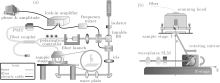
The system consists of a commercial SNOM (NT-MDT) and a home-built Mach– Zehnder interferometer, as shown in Fig. 2. A laser beam with the wavelength of 633 nm is divided into two beams by a tunable beam splitter. The two beams pass through two AOMs driven by a frequency generator (IntraAction DFE-404A4) at 40 MHz and 40.02 MHz respectively. Iris is used to choose the + 1 order from the diffracted beams. Due to the frequency shift between the reference and the object arms, a 20 kHz beat signal is generated. The optical field at the sample surface is collected with a commercial aluminized aperture fiber probe produced by NT-MDT. The aperture diameter is about 50– 100 nm with a transmission coefficient of 10− 4. Since the signals collected by the probe are pretty weak, the quality of the interference signals must be guaranteed by adjusting the splitting ratio. To obtain a better interference contrast, a 3-paddle fiber polarization controller (Thorlabs FPC560) is used in the reference arm to make sure that the long axes of the two polarization ellipses are parallel. The three paddles are configured to approximate quarter-wave, half-wave, and quarter-wave plates when used at the design wavelength. We adjust these paddles to maximize the interference contrast. The signals detected by PMT (Hamamatsu H5784) contain the field parameter information we need. The 20 kHz signal working as the lock-in reference is provided by a frequency mixer, which can be obtained by directly mixing the two driving frequencies from the AOM generator. Using a lock-in amplifier to demodulate the signals at the beat frequency, the phase and amplitude are recovered.
To decrease the phase drift, the optical lengths of the object and the reference arms should be equal. The phase is much more sensitive to the environmental change compared with the intensity. A bigger optical path difference leads to a larger phase drift when disturbed by the external environment. Minimizing the optical path helps to improve the system stability. All of the fiber connectors are welded by a fiber fusion splicer to increase the transmission efficiency.
Figure 2(b) shows the illumination platform. A rotating mirror is attached on a slider of the X stage. The mirror can rotate in the X– Y plane and move along the X axis driven by electric motors. The positioning accuracy is 0.01° and 1 μ m, respectively. Many SPP devices are illuminated and excited with different incident angles, meanwhile the incident spot must remain intact.[16, 17] Different incident angles correspond to different rotating angles and positions of the mirror. A data table is made in advance to record their matching relations. With an operating software written in LabView, the system can automatically adjust the rotating angle and the position to satisfy the incident angle and keep the spot within 0.2 mm. When scanning, the probe is driven by the pizeo-actuator embeded in the scanning head. The max scanning area can be as large as 100 μ m× 100 μ m. Besides, by adjusting the waveplates and the spatial light modulator (SLM), circular, linear, radial, and azimuthal polarizations can be realized to satisfy various measure requirements.
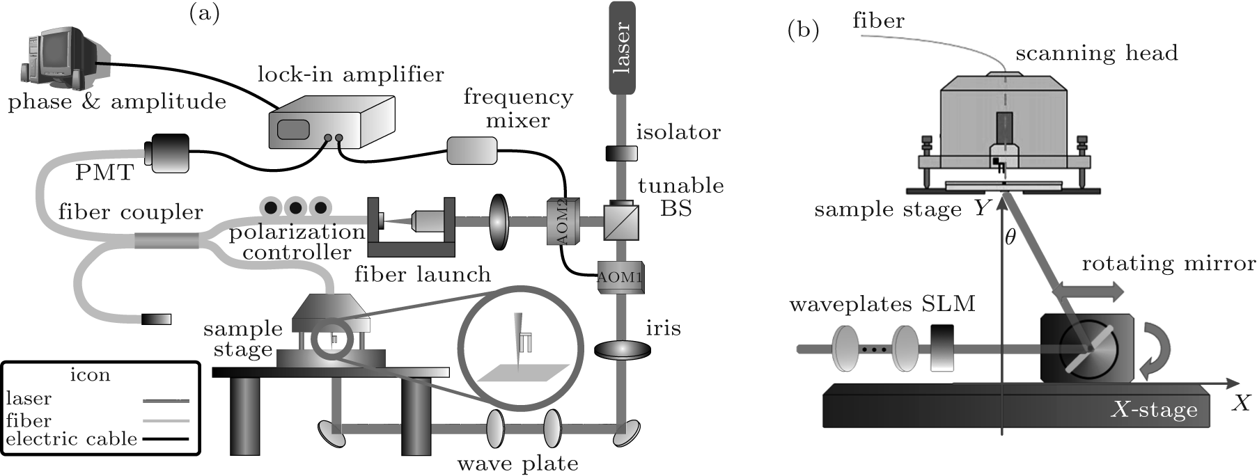 | Fig. 2. Setup of phase sensitive SNOM: (a) schematic diagram of the near-field heterodyne interferometry phase detecting system, (b) illumination platform. It can adapt to different incident angles and polarization requirements with high stability. |
4. Results
4.1. Phase grating
A pure phase grating is introduced to test the system. The grating constant is 600 lines per millimeter, the period is about 1.67 μ m. Figure 3(a) is the three-dimensional (3D) topography of the grating. Figures 3(b)– 3(d) are synchronously measured topography, optical amplitude and phase distributions, respectively. They have perfect corresponding relationships with each other. The measured period is about 1.7 μ m, which shows a good agreement with the nominal grating constant. It is noticed that the phase distribution is continuously changed from − π to π .
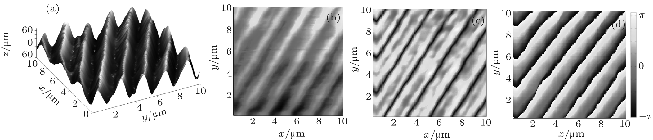 | Fig. 3. Measured topography and optical field distributions of a phase grating: (a) 3D topography, (b) topography, (c) amplitude, (d) phase. |
With the phase-sensitive SNOM, any cross section of an optical field formed by irregular phase modulation surfaces can be obtained, which has a prospective application on studying photonic crystals, optical waveguides, phase singularities, etc.
4.2. SPP interference
Although there have been several phase detection methods, reports on SPP phase mapping are still rare in the visible range. Since SPPs are highly confined in the near field region and the dominate components of their electric fields are in plane, the aperture fiber probe shows its advantage in detecting SPPs.
We fabricate 10 column grooves, with L = 40 μ m, W = 300 nm, and D = 10 μ m, on a 150 nm-thick gold film using focused ion beam (FIB), as shown in Fig. 5(c). Polarized 633-nm He– Ne laser light is vertically focused on the back of the sample and excites SPP waves on the sample surface. The propagation of the SPPs is investigated using the home made phase sensitive SNOM. Figures 4(a) and 4(b) are synchronously obtained optical amplitude and phase distributions of a single groove, respectively. The propagation characteristics of the SPPs are inconspicuous in the intensity distribution. While the phase distribution shows quite strong and rapid changes and reveals much more information. The wavelength of SPP is given by
which shows that the SPP wavelength is a function of the free space wavelength λ 0. Here 
 | Fig. 4. Measured and simulated optical field distributions of SPP grooves: (a)– (c) single groove, (d)– (f) twin grooves. |
 | Fig. 5. Sample description and principle of SPP excitation. Panels (a) and (b) illustrate how different incident polarizations interact with the gold groove and generate SPP waves. Panel (c) is the description of the groove sample. |
5. Discussion
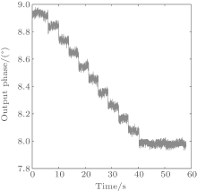
The phase resolution of the signal acquirement and processing electric system is tested by inputting two signals with the same frequency. The two signals with different initial phases are generated by a digital signal generator (Agilent 33522A). The phase delay between the two signals can be manually adjusted with an accuracy of 0.01° . These two signals can be regarded as the heterodyne signal and the reference signal provided by PMT and the frequency mixer in Fig. 2(a). Figure 6 shows the results of the phase resolution. When the input phase delay is changed by a step of 0.1° , via the lock-in amplifier (Perkin Elmer 7280) and the synchronizing system, such small changes can be clearly distinguished from the final phase output. The electric processing system has a resolution better than 0.1° .
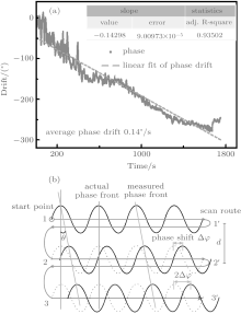
Before the measurement, we need to test the phase stability and drift of the system. Remove the sample and let the object beam directly illuminate on the probe, we display in Fig. 7(a) the typical phase measurements after 2 h and for a time duration of 30 min. The phase drift is almost linear. From our experience, the variation of the refractive index in the optical path has a great effect on the phase drift. Eight thermometers are distributed at different positions as monitors. When the interferometer starts to heat up, the temperature is changed and this leads to a thermal gradient. The temperature change and air flow cause the refraction index to change. The greater the optical path difference between the reference and the object arms, the bigger the phase drift. The spatial light path and fiber light path in the two arms should be equal; however, it is rather difficult to realize, thus we can only minimize the drift to a particular level.
 | Fig. 6. Phase resolution of the electric system. When the input phase delay is decreased by 0.1° , the change in the output phase can be easily distinguished. |
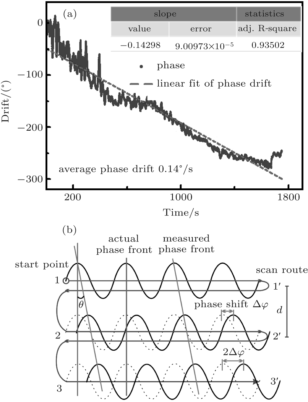 | Fig. 7. Phase drift and rotation error: (a) measured phase drift during 30 min, (b) rotation error caused by phase drift. |
In Fig. 7(a), the blue curve indicates the phase variation with time in the experiment. The red dot line is the linear fit of the phase drift with a slope of − 0.143, which indicates that the average phase drift is 0.14° /s. The time constant of the lock-in amplifier is 2 ms. The sampling time is 10 ms per point. For a 10 μ m × 10 μ m area, the scan frequency is 1 s per line. The phase drift does not have much change on the field distribution, only a small rotation occurs on the image. Figure 7(b) illustrates how the phase drift induce this rotation. The scan route described in blue follows 1– 1′ – 2– 2′ – · · · n′ . For a certain line, every point has a Δ φ phase delay compared with the previous line. The dashed sinusoidal line represents the actual phase, the solid black line stands for the measured phase. Suppose that the actual equal phase front is linked by the red lines, while the measured equal phase front is the green lines. There is a rotation error θ between the actual and the measured equal phase fronts due to phase shift Δ φ

Here L is the length of the scan area N is the number of sampling points per line, and n is the number of phase periods per line. In the grating case, L = 10 μ m, N = 100, n = 5. Substituting into formula (3), θ is about 8.9× 10− 3 degree. Depending on the size of the scanning area and the resolution, it usually takes about 5– 15 min to complete the mapping of one image. The effect of the phase drift may be negligible in such a small scan time. Since the phase drift is regular, a compensative processing can be conducted simply by adding a 0.14T degree for each point of the phase, where T is the instantaneous time of the present point. The spatial resolution is high enough for reconstructing the phase front distribution. The phase accuracy can be described as the standard deviation of the measured phase. According to the measured data in Fig. 7(a), the phase accuracy is about λ /36 (10° ) calculated by MATLAB, which is precise enough for phase distribution mapping of SPP waves.
6. Conclusion
We demonstrate the principles and the setup of a novel phase-sensitive SNOM based on an aperture fiber probe and the heterodyne interferometry. It combines a spatial optical path and a fiber optical path working at the visible spectrum, and can synchronously map topography, optical phase and amplitude distributions. The spatial optical path works for illumination is flexible to meet the complex illumination and excitation requirements, while the fiber path is more stable and disturbance proof for signal transmission.
Two kinds of basic nano-photonic devices are investigated in this article. With the phase-sensitive SNOM, any cross section of the optical field formed by irregular phase modulation surfaces can be obtained. It has many promising applications on SPP devices. The phase distribution and the interference pattern will enable us to gain a better understanding of how light interacts with SPP structures and how SPP waves propagate in plane. At last, the phase resolution, the accuracy, and the drift of the system and its effect on mapping results are discussed. The phase resolution can be as high as 0.1° with an accuracy of 10° . This phase-sensitive SNOM is a powerful tool for phase distribution mapping and has a significant guidance on nano-photonic device design and optimization.
Reference
| 1 |
|
| 2 |
|
| 3 |
|
| 4 |
|
| 5 |
|
| 6 |
|
| 7 |
|
| 8 |
|
| 9 |
|
| 10 |
|
| 11 |
|
| 12 |
|
| 13 |
|
| 14 |
|
| 15 |
|
| 16 |
|
| 17 |
|
| 18 |
|