Ghost imaging based on Pearson correlation coefficients*
[Yu Wen-Kaia), b) , Yao Xu-Ria), b) , Liu Xue-Fenga) , Li Long-Zhena), b) , Zhai Guang-Jieb)†  ]
]
]
|
|


†Corresponding author. E-mail: gjzhai@nssc.ac.cn
*Project supported by the National Key Scientific Instrument and Equipment Development Project of China (Grant No. 2013YQ030595) and the National High Technology Research and Development Program of China (Grant No. 2013AA122902).
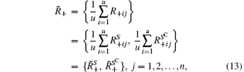
Correspondence imaging is a new modality of ghost imaging, which can retrieve a positive/negative image by simple conditional averaging of the reference frames that correspond to relatively large/small values of the total intensity measured at the bucket detector. Here we propose and experimentally demonstrate a more rigorous and general approach in which a ghost image is retrieved by calculating a Pearson correlation coefficient between the bucket detector intensity and the brightness at a given pixel of the reference frames, and at the next pixel, and so on. Furthermore, we theoretically provide a statistical interpretation of these two imaging phenomena, and explain how the error depends on the sample size and what kind of distribution the error obeys. According to our analysis, the image signal-to-noise ratio can be greatly improved and the sampling number reduced by means of our new method.
In traditional ghost imaging (GI), an optical source generates a signal beam and a reference beam at a beam splitter; the signal beam is used to illuminate an object, after which its total intensity is collected by a bucket detector with no spatial resolution; in the other arm the spatial distribution of the light is measured by a high spatial-resolution detector. Neither detector can “ see” the object on its own, but a “ ghost” image can be retrieved by cross correlating the outputs of the two detectors. The initial experimental demonstration of GI used the entangled signal and idler photons generated from spontaneous parametric downconversion, [1, 2] hence ghost image formation was ascribed to the quantum entanglement of the photons.[3] A controversy soon arose, however, when theory[4] and experiment[5, 6] showed that GI is also achievable with pseudo-thermal light obtained by passing a laser beam through a rotating ground-glass diffuser, or with true thermal light.[7] This sparked a warm discussion on the nature of thermal light GI.[8, 9] As a consequence, GI with a classical source aroused the interest of many groups and developed numerous branches, such as computational GI, [10] compressive GI, [11] differential GI, [12] optical encryption, [13] adaptive compressive GI, [14] and lensless GI with sunlight.[15]
In particular, Luo et al.[16, 17] found a seemingly completely nonlocal form of imaging in which conditional averaging of the reference measurements could improve the image visibility with fewer exposures and reduced computation time. They called this technique correspondence imaging (CI). However, no strict analytical proof was provided. Soon after, Wen[18, 19] offered some theoretical explanations on their findings, while Shih et al.[20] suggested a quantum interference model. However, Ref. [20] failed to show why negative images can be formed in thermal CI, or why the visibility can be substantially improved beyond the 1/3 limit for thermal light second-order correlation. In contrast, these were explained to some extent by Wen in Refs. [18] and [19]. This CI method further demonstrates the importance of intensity fluctuations in nonlocal imaging with thermal light.[21, 22] Later, in Ref. [21], Yao et al. also gave a statistical optics model to explain this CI phenomenon. Further experimental and theoretical developments of this positive-negative image concept have been presented in many other papers.[23– 26] In this paper, we present a new statistical explanation which we hope provides deeper insight into the essence of CI. Moreover, on the basis of this interpretation, we propose a more rigorous and standard analysis of GI where a ghost image can be obtained by calculating a Pearson correlation coefficient between the bucket detector intensity and the brightness at a given pixel of the reference detector, then for the next pixel and the next, and so on. This method further answers what kind of distribution the error obeys and how the error depends on the sample size, i.e. the number of measurements.
This paper is organized as follows. In Section 2, we experimentally demonstrate ghost imaging based on Pearson correlation coefficients (GIPCC) in a computational GI scheme and present some results to compare its performance with other GI reconstructions. Then, in Section 3, we give a statistical analysis of CI positive-negative image formation and an explanation of our imaging approach. We show that the values recorded by a bucket detector play the role of a selection criterion in CI, and can also be used to calculate the correlation coefficients between the bucket brightness and the brightness at each pixel of the frames. Our analysis thus casts doubt on whether CI is a rigorous and standard approach to obtain ghost images, while demonstrating that GIPCC is a better way of reconstructing binary objects with high image quality and fewer measurements. Finally, in Section 4, we briefly summarize this work.
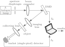
Our experiment is based on computational GI, as shown in Fig. 1. The advantage of computational GI is that it can be performed without a high spatial resolution detector, and it only needs to pre-compute the spatial distribution after a wide range of free space propagation distances. Here we use a digital micromirror device (DMD) consisting of 1024 × 768 micro-mirrors each of size 13.68 × 13.68 μ m2, rather than a spatial light modulator, to generate random spatial distributions. Each mirror can be oriented at + 12° and − 12° away from the initial position, thus the light falling on it will be reflected in two directions. The frame frequency (modulation frequency) of the DMD is up to 32552 Hz. In our experiment, the light from a halogen lamp of 55 W power is projected onto the DMD, first passing through an aperture diaphragm and a beam expander. Random binary patterns are encoded onto an area of 160 × 160 micromirrors (pixels) of the DMD. We image these random patterns IR onto an object which is a black-and-white film printed with “ A” . Only the light reflected from the micromirrors oriented at + 12° is projected onto the object. Then a convex lens is used to collect the corresponding total light intensity IB into a bucket (single-pixel) detector. Here we use a 1/1.8 in. charge-coupled device (CCD) with 1280 × 1024 pixels and an exposure rate of 26 frames per second as the bucket (single-pixel) detector, by integrating the gray values of all the pixels in each exposure. A ghost image of the object can be reconstructed by cross correlating the random binary patterns IR with the bucket intensity IB.
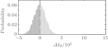
The recorded total intensity IB from the bucket detector is random because of the random modulation of the DMD and the purely stochastic intensity fluctuations of the thermal light source. We calculate Δ IB = IB – 〈 IB〉 , then plot the probability distribution of Δ IB. By using 〈 IB〉 as a boundary, we divide {IB} into two subsets:


which contribute to the left and right half of Fig. 2.
 | Fig. 1. Experimental setup for computational GI. A halogen lamp illuminates the DMD through an aperture diaphragm and a beam expander. The reflected random patterns are imaged onto an object which is a black-and-white film printed with “ A” and then collected by a bucket (single-pixel) detector. IR: binary random patterns encoded on the DMD. IB: total intensity recorded by the bucket (single-pixel) detector. |
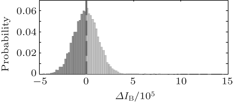 | Fig. 2. Probability distribution of Δ IB, where Δ IB = IB – 〈 IB〉 . The left side (blue) is binned for Δ IB < 0, and the right side (pink) for Δ IB > 0. The dashed line denotes 〈 Δ IB〉 . |
Statistically, each element of the average matrix 〈 IR〉 is a constant, which only reveals the intrinsic fluctuations of the lamp source hitting this pixel, rather than any information about the object. Amazingly, according to Luo’ s method, after the partition, a positive (or negative) correspondence image can be retrieved by only averaging the IR frames corresponding to B+ (or B− ), identified by the subscript “ + ” (or “ − ” ):


Actually, artificially dividing the 〈 IR〉 into R̄ + and R̄ − is not standard, so is not optimal. Moreover, Luo’ s procedure could not answer what kind of distribution the error obeys, and how the error depends on the sample size. In this letter, we wish to report another interesting imaging approach based on Pearson correlation coefficients to answer these questions.
First, we flatten the two-dimensional image pixel matrix into a one-dimensional column vector, and denote it by x. Our starting equation is

where B is m × 1, R is m × n, x is n × 1, m is the sample size (total number of frames), and n is the total number of pixels. Each pattern distribution can be shaped into a row vector, then m random distributions can be rearranged row by row into a measurement matrix R. That is, each row of R records the brightness of pixels in one frame. As performed in the experiment, the actual random patterns sequentially fed into the DMD only have two values, 0 or 1, corresponding to the ± 12° angles at which the micromirrors are deflected.
For simplicity, here we only consider a binary object mask, either transparent (1) or opaque (0). The simplest model of GI is the probabilistic one: a transparent pixel correlates with the bucket signal while an opaque pixel is independent of the bucket signal. The principle of CI is that the frames with above-average bucket signals correspond to a good overlap between the reference frame and the transparent object, while those with below-average signals tend to have a good overlap with the opaque object. Here we give a more intuitive picture of the preference for a transparent pixel (i.e. imaging) as follows. The definition of a Pearson correlation coefficient (which is just a number) is well known.[27] Here we calculate the sample Pearson correlation coefficient rj (corresponding to a pixel j in x) between B and a column vector Rj of R. The coefficient rj is given by
where cov is the covariance, σ the standard deviation, and − 1≤ rj ≤ 1, j = 1, 2, … , n. A positive (negative) value of rj means a positive (negative) linear relationship, while rj = 1 or − 1 occurs only when all the points of the scatter plot lie exactly on a straight line. The value 1 denotes total positive correlation, 0 no correlation, and − 1 total negative correlation. Thus rj measures only the linear relationship between Rj and B, j = 1, 2, … , n. If rj is significantly greater than 0, then pixel j is coded as 1 (transparent). After j calculations, we will obtain a sequence vector r of length n, then we reshape this one-dimensional vector back to a two-dimensional array of υ × ν pixel size, where υ × ν = n. This array is the image recovered by GIPCC, which regards each sample Pearson correlation coefficient rj as the j-th pixel of the image.
For a quantitative comparison of the image quality, we introduce the peak signal-to-noise ratio (PSNR) and the mean square error (MSE) as figures of merit

where 
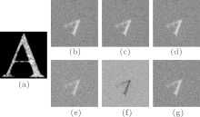
To check the quality of GIPCC, we made a comparison of GIPCC with other GI approaches. Figure 3(a) shows a direct image of the object illuminated by random DMD patterns, taken by a CCD camera. The reconstructions of GIPCC, background-subtracted correlation function Δ GI = 〈 IRIB〉 – 〈 IR〉 〈 IB〉 , and the normalized correlation function 
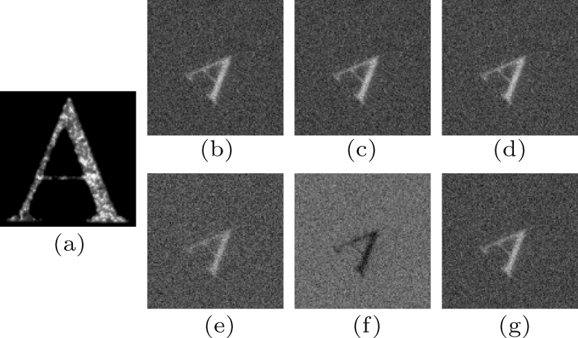 | Fig. 3. Comparison between GIPCC and other conventional GI techniques which reconstruct the full 160 × 160 pixel image. All figures are automatically gray-scale compensated. (a) The direct image of the object. (b)– (d) Images retrieved by GIPCC, Δ GI, and g2 with 11940 patterns and a PSNR of 8.312, 8.311, and 8.188 dB, respectively, (e) and (f) are R+ positive and R− negative correspondence images, from 5882 and 6058 patterns, with PSNRs of 7.425 and 5.562 dB, respectively, (g) is the image Δ G obtained by averaging all 11940 patterns but with G− inverted, with a PSNR of 8.088 dB. |
In mathematics, the support of a function is the set of points where the values are not zero. Suppose that the object x has k nonzero entries, and define its support set as S, where | | S| | 0 = k. Here the l0 norm is defined as 
Let us recall the initial second-order correlation function G(2) = 〈 IR〉 〈 IB〉 where the bucket signal can be treated as weights. When all the elements in B are the same constant c, G(2) turns out to be cR̄ which in fact cannot reflect any information of the object. If we normalize this bucket signal to a binary sequence taking two values “ 1” and “ 0” (B ≥ B̄ for “ 1” , and B < B̄ for “ 0” , or vice versa), then we will get a positive (or negative) image with high image quality. Thus CI is indeed amazing in that it can transform the poor performance of an initial second-order correlation into a good one. Here we build a model to further explain this phenomenon. We have the conditional probability for B±

and the total probability formula

where B± is for ± (B – B̄ ) > 0 and Γ ± = ∫ B± P(B)dB > 0. Denote the mean of P± (R) and P(R) by R̄ ± and R̄ , respectively,
so (R̄ + – R̄ ) and (R̄ − – R̄ ) have opposite signs. The terms in 〈 (R – R̄ )(B – B̄ )〉 are of two forms indexed by ± . The one in support set S indexed by + is
The terms with + replaced by − have the same sign. Since the two factors (B̄ + – B̄ ) and (B̄ − – B̄ ) both have opposite signs from that of the ± term, we have 

The column vector Rj can be treated as a time sequence of reference light field intensities, and each element in B can be seen as the inner product of each modulation pattern and the object. Notice that R of the DMD is a binary matrix consisting of the two values 0 or 1, thus B reflects the sum of the pixel spot brightnesses, and the probability of B involves the convolution of the probability of single pixel brightness (Rij of frame i at pixel j). To avoid the operation of convolution, a natural assumption is: the summation over k transparent pixels of the object mask is equivalent to the summation over k frames at a single pixel of the DMD. The brightness at all pixel spots has an identical distribution P(Rij). For transparent pixels, we may decompose 

Taking the k-th root of the Laplace transformation of F+ (R), and then making a back-Laplace transformation will give the required conditional distribution for a single pixel, which will be denoted as P+ (Rij). However, we do not need this explicit form. As mentioned before, we have proved that the mean of 
To demonstrate this more clearly, we assume | | B+ | | 0 = u, and | | B− | | 0 = v, and define SC as the complementary set of S, which stands for opaque pixels, then we have

Since 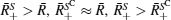


A key advantage of our GIPCC method is the ability to fill the gap and solve these problems. For pairs from an uncorrelated bivariate normal distribution, the sampling distribution of Pearson’ s correlation coefficient follows the Student’ s t-distribution with degrees of freedom (m − 2): 

where “ ln” is the natural logarithm function and “ arctanh” is the inverse hyperbolic function. Here (Rj, B) has a bivariate normal distribution, and the (Rij, Bi) pairs used to form rj are independent for i = 1, … , m, then z approximately follows a normal distribution with mean z and standard variation 
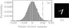
For a binary object mask, the gray value takes on either “ 1” or “ 0” . Taking Fig. 3(b) for example, the number of sampling patterns is 11940, so the background error approximately follows a normal distribution with mean 0 and standard variation 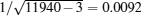
 | Fig. 4. Results of hypothesis testing. (a) Probability distribution of the error samples. The location of the critical value is identified by the red dashed line. (b) Retrieved image based on statistical hypothesis testing, with a PSNR of 16.301 dB. |
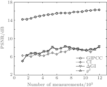
In the model of independent pixels, the correlation between a transparent pixel and the bucket is r(Rt, B) ∼ t− 1/2, where t is the total number of transparent pixels. If r is small, Fisher’ s transformed variable is roughly F ∼ t− 1/2. Since the variance of Fisher’ s variable is σ ∼ m− 1/2, where n is the total number of sampling frames, it is required that F(r) ≫ σ , or m ≫ t. Therefore, if the object is sparse (like the film used in our experiment), the number of measurements in GIPCC will be dramatically reduced. To further demonstrate this advantage of GIPCC, the PSNR values of GIPCC and other conventional GI techniques against the number of measurements are given in Fig. 5. We can see clearly that the image quality obtained by various methods is approximately proportional to the number of measurements. The PSNRs of GIPCC are always better than other GI approaches, thus the number of measurements in GIPCC is much smaller than that in other GI methods for the same PSNR value, which agrees with our theory.
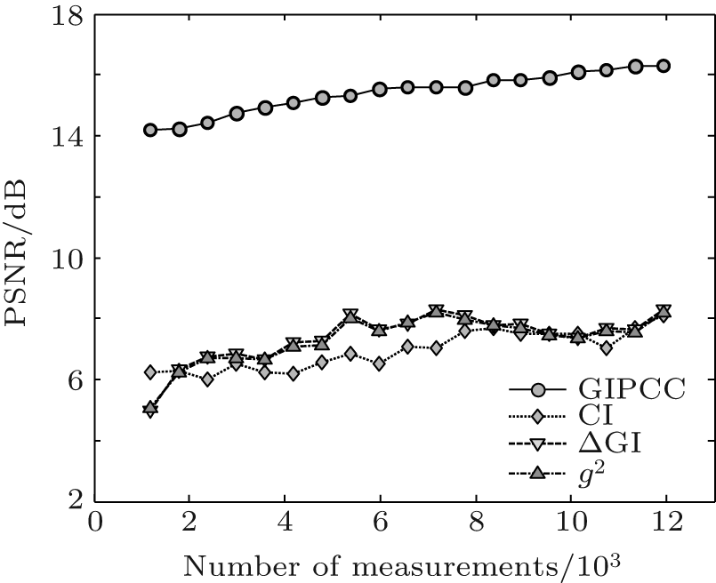 | Fig. 5. PSNR values of GIPCC and other conventional GI techniques versus the number of measurements. |
Now let us analyze the image formation in our GIPCC method. Without loss of generality, consider a and b are of zero mean and unity variance. Then, the correlation between a and b is 

where b+ ≥ 0 and the conditional mean values as


Therefore,
Thus, either both ā ± vanish, or they have opposite signs. Similarly, from 〈 b〉 = 0 we have

We now prove by reduction to absurdity that if r = 0 then ā + = ā − = 0. By representing (ā + , ā − ) and (


In conclusion, we have improved the correspondence imaging technique by developing an alternative method to reconstruct the image, whereby each pixel of the image is acquired by calculating a Pearson correlation coefficient between the bucket intensity and the brightness at each pixel of the DMD modulation patterns. This method illustrates how the error depends on the sample size and what kind of distribution the error obeys, and thus can be seen as a more rigorous and general approach compared with the original correspondence imaging scheme. We have experimentally demonstrated our method in a computational ghost imaging setup with thermal light, and have obtained a much better peak signal-to-noise ratio compared with other ghost imaging approaches. Furthermore, we have provided a theoretical analysis and intuitive interpretation of the formation of the positive– negative image in correspondence imaging. This new protocol offers a general approach applicable to all ghost imaging techniques. The applications include but are not limited to remote sensing, positioning, and imaging.
We are grateful to Wei-Mou Zheng for the illuminating discussion on the topic presented here. We warmly acknowledge Kai-Hong Luo and Ling-An Wu for providing suggestions, encouragement, and helpful discussion.
| 1 |
|
| 2 |
|
| 3 |
|
| 4 |
|
| 5 |
|
| 6 |
|
| 7 |
|
| 8 |
|
| 9 |
|
| 10 |
|
| 11 |
|
| 12 |
|
| 13 |
|
| 14 |
|
| 15 |
|
| 16 |
|
| 17 |
|
| 18 |
|
| 19 |
|
| 20 |
|
| 21 |
|
| 22 |
|
| 23 |
|
| 24 |
|
| 25 |
|
| 26 |
|
| 27 |
|
| 28 |
|
| 29 |
|
| 30 |
|