


Influence of obstacle on electromagnetic wave propagation in evaporation duct with experiment verification*
[Shi Yang, Kun-De Yang , Yang Yi-Xin, Ma Yuan-Liang]
, Yang Yi-Xin, Ma Yuan-Liang]
 |


†Corresponding author. E-mail: ykdzym@nwpu.edu.cn
*Project supported by the National Natural Science Foundation of China (Grant No. 11174235) and the Fundamental Research Funds for the Central Universities of China (Grant No. 3102014JC02010301).
In this paper, the influence of obstacle on electromagnetic wave propagation in an evaporation duct is investigated, both from numerical simulation and experimental observation. A comparison of electromagnetic wave propagation in evaporation duct with and without obstacle for a typical case is presented. The presence of obstacle causes a significant increase in path loss. The obstacle has significant impact on electromagnetic wave propagation when the frequency is higher than 5 GHz and when the evaporation duct height is higher than 10 m. The influence of an island on electromagnetic wave propagation was observed in the experiment held in the South China Sea, October 2012. The experiment result shows that the island causes about 30–40 dB increase in path loss. The discrepancy between model and measurement is analyzed and the errors of transmitting antenna height and relative humidity are the possible causes of the discrepancy.
An evaporation duct forms in the atmospheric surface layer due to the gradual decrease of humidity from the ocean surface upwards.[1] The trapping layer of the evaporation duct behaves like a waveguide and can lead to a decreased path loss at microwave bands, and extend radar detection range and communication range.[2, 3] The evaporation duct has been recognized as a propagation mechanism that can result in substantially stronger signals over-the-horizon paths above the ocean surface at microwave bands.[4– 6] As a result, the propagation characteristics of electromagnetic wave in the evaporation duct are significant in determining the performance of ship-borne radar and communication systems.
One of the propagation problems is that the propagation path is sometimes blocked by obstacles, such as a ship or an island. Numerical methods[7– 10] have been proposed to simulate the electromagnetic wave propagation over terrain using parabolic wave equation. However, the influence of obstacles on electromagnetic wave propagation in the evaporation duct and, especially, experimental studies have been reported seldomly.
The purpose of this work is to investigate the influence of an obstacle on electromagnetic wave propagation in an evaporation duct both from numerical simulation and experimental observation. A comparison of the electromagnetic wave propagation in evaporation duct with and without an obstacle for a typical case is presented in Section 2. Then, the influences on electromagnetic wave of different frequencies and with different evaporation duct parameters are discussed. In Section 3, the evaporation duct experiment held in the South China Sea in 2012 is presented and the data collected are used to verify the conclusion. The discrepancy between model and measurement is analyzed in detail.
The wedge obstacle model used in the simulation is shown in Fig. 1(a). The obstacle’ s height and width are 20 m and 4 km, respectively. It is located at 50 km away from the transmitting antenna. A neutral evaporation duct condition is used in the simulation (air temperature: 20 ° C, sea surface temperature: 20 ° C, relative humidity: 65%, wind speed: 8 m/s, pressure: 1022.2 hPa). The modified refractivity profile calculated by the Naval Postgraduate School (NPS) model[11] is shown in Fig. 1(b). The evaporation duct height is 15.8 m.
The electromagnetic wave propagation in an evaporation duct with an obstacle is a complicated physical problem. The refraction and diffraction of electromagnetic wave should be considered. As the atmospheric refraction environment and the boundary condition are usually complicated, numerical methods such as ray trace method, parabolic equation method (PE), and hybrid method are usually used to solve the equation.
The parabolic equation method has been widely used to calculate electromagnetic wave propagation in the troposphere. The advantage of the PE method is that it can simulate electromagnetic wave propagation in a range-dependent troposphere environment with variable terrain. The standard parabolic equation can be obtained from the Helmholtz equation under certain assumptions as

where u represents a scalar component of the electric field for horizontal polarization or a scalar component of the magnetic field for vertical polarization, z is the height, x is the range, k0 is the free space wave number, and m is the modified refractive index.
 | Fig. 1. Numerical simulation condition: (a) the wedge obstacle model; (b) the modified refractivity profile. |
Let u(xk, z) be the complex scalar component of the field at range xk and height z. Then, the field at range xk + 1 and height z, denoted by u(xk+ 1, z), can be given by the Fourier split-step solution of PE
 | (2) |
where F[· ] and F− 1[· ] are the Fourier transform and the Fourier inverse transform, respectively, p is the transform variable, and δ x is the range increment, defined by δ x = xk+ 1 − xk. Detailed information about Fourier split-step PE solution can be found in Refs. [12]– [14].
The APM model is a hybrid model which combines radio physical optics (RPO) and terrain parabolic equation model (TPEM) in a relative fast code. It allows both horizontal and vertical variation in modified refractivity along the propagation path over terrain. The APM model is used in advanced refractivity effects prediction system (AREPS), [12] which is widely used for the assessment of electromagnetic systems. It has also been validated in various terrain and evaporation duct environments.[14, 15] Thus, the APM model is used to study the electromagnetic wave propagation with an obstacle in evaporation duct in this paper. The terrain profile and the modified refractivity profile are input into the APM model to calculate the path loss. The transmitting antenna height is assumed to be 3 m and the electromagnetic wave frequency is 8 GHz. The polarization of the wave is horizontal. The propagation distance is 100 km in the simulation.
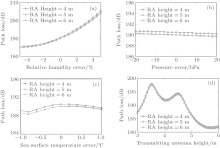
 | Fig. 2. Path loss distribution of electromagnetic wave propagation in evaporation duct: (a) without the obstacle; (b) with the obstacle; (c) path loss at 100 km. |
Figure 2 shows the comparison of the path loss distribution with and without the obstacle. It is obvious from Fig. 2 that the obstacle has significant impact on the electromagnetic wave propagation in evaporation duct. Figure 2(b) shows that there is an obvious shadow region behind the wedge obstacle. Figure 2(c) shows a comparison of path loss at the range of 100 km with and without obstacle. The path loss at the height of 5 m is about 135 dB without the obstacle, while the path loss is about 181 dB with the obstacle. The obstacle causes about 46 dB increase in the path loss.
Figure 3(a) shows the influence of obstacle on electromagnetic wave propagation with different evaporation duct parameters. The input parameters of APM model are shown in Table 1 (Case 1) and the evaporation duct height (EDH) changes from 6.5 m to 20.7 m. When the EDH is below 8 m, the path loss with obstacle is only several decibels higher than that without obstacle at 8 GHz. The obstacle has a larger impact on electromagnetic wave propagation when the EDH is higher than 10 m. For example, when the EDH is 14 m, the path loss with the obstacle is about 30– 40 dB higher than that without obstacle. That is to say, the influence of obstacle becomes significant when the EDH is high.
The influence of obstacle on electromagnetic wave propagation of different frequencies is shown in Fig. 3(b). The input parameters of APM model are shown in Table 1 (Case 2) and the frequency changes from 1 GHz to 20 GHz. When the electromagnetic wave frequency is lower than 4 GHz, the path loss with obstacle is about 3 dB higher than that without the obstacle. However, when the frequency is higher than 5 GHz, the obstacle begins to impact the electromagnetic wave propagation significantly. The path loss with the obstacle becomes 30– 60 dB higher than that without the obstacle. The largest impact of the obstacle is at the frequency of 11 GHz and 16.5 GHz, which shows a difference of about 90 dB. That is to say, the impact of obstacle on electromagnetic wave propagation becomes significant when the frequency is high.
| Table 1. Input parameters of the APM model. |
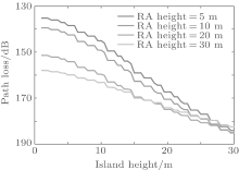
Figure 4 shows the influence of obstacles with different height on electromagnetic wave propagation. The input information is shown in Table 1 (Case 3) and the obstacle’ s height changes from 0 m to 30 m. When the receiving antenna height is 5 m, the path loss is about 135 dB without the obstacle. The path loss (receiving antenna height 5 m) increases by about 8– 10 dB when the obstacle’ s height increases every 5 m. The path loss increases to about 185 dB when the obstacle’ s height is 30 m. It can also be concluded that the obstacle has a larger impact on the path loss with lower receiving antenna height. For example, when the obstacle height is 15 m, the path loss at the height of 30 m is about 170 dB, which is only 10 dB higher than that without the obstacle. While the path loss at the height of 5 m is about 160 dB, about 25 dB higher than that without the obstacle.
 | Fig. 3. Influence of obstacle on electromagnetic wave propagation: (a) different evaporation duct parameters; (b) different frequencies. |
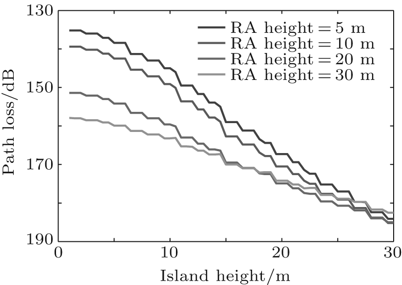 | Fig. 4. Influence of obstacle on electromagnetic wave propagation at different obstacle’ s heights. |
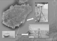
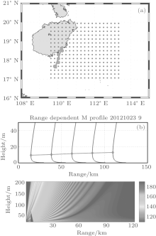
The experiment was held in the South China Sea in October 2012. The transmitting antenna was located in Ri Yuewan (18.6283° N, 110.2133° E) in Hainan Province. The receiving antenna was installed on a research vessel (see Fig. 5). The research vessel sailed on the north part of the South China Sea. The propagation path was sometimes blocked by islands or ships during the experiment and the influence of the obstacle on electromagnetic wave propagation was measured.
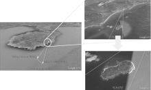
On 23 October 2012, the microwave signal transmitted from Ri Yuewan was received on the research vessel. From about 9 a.m. to 10 a.m. (UTC+ 8), the propagation path was blocked by the island which is located at about 5 km away from the transmitting location (Fig. 6). The receiving signal level was recorded during this process. The experiment conditions are described in Table 2.
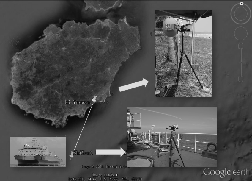 | Fig. 5. Evaporation duct experiment location. |
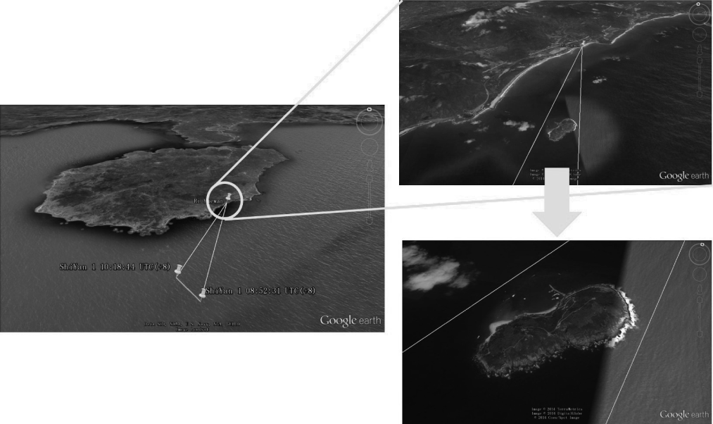 | Fig. 6. Propagation path was blocked by the island. |
| Table 2. Experiment conditions on 23 October 2012. |
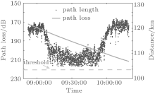
Figure 7 shows the influence of the island on electromagnetic wave propagation measured in the experiment. It is shown that the path loss was about 170– 180 dB without the island. When the island begins to block the propagation path, the path loss increases to about 200 dB and remains at 200– 210 dB. At 10:00 a.m., the propagation path has not been blocked by the island and the path loss returned back to about 175 dB. Thus, the island causes an increase of about 30– 40 dB in the path loss. The length of propagation path changed from 122 km to 107 km in this process. The measurement was repeated on 25 October 2012. The result is similar to the measurement on 23 October and the obstacle also caused about 30– 40 dB increase in path loss. The data measured on 23 Oct are used to verify the model’ s result.
 | Fig. 7. Path loss measured in the experiment. |
The 9:35 a.m. (UTC+ 8) is selected to verify the model calculation. At 9:35 a.m., the research vessel was at 17° 38′ 10.80″ N 109° 53′ 0.24″ E, 125 km away from the transmitting location. Figure 4 shows the propagation path at this time. The terrain profile is obtained from the Google earth, which is shown in Fig. 8. The height of the island is about 55 m and the width of the island is about 1 km. The island is at about 5 km away from Ri Yuewan.
 | Fig. 8. (a) Topography of the island. (b) The terrain profile of the island. |
The NCEP CFSR reanalysis data[16, 17] (9:00(UTC+ 8), 23 October 2012) are used to get the atmosphere factors and the NPS model is used to calculate the modified refractivity profile along the propagation path as shown in Fig. 9(a). The evaporation duct height is about 12 m along the propagation path (Fig. 9(b)).
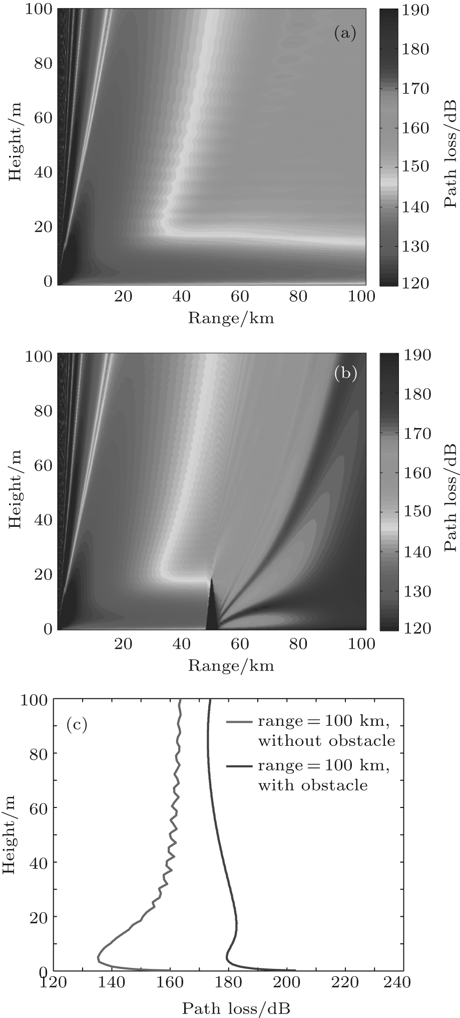
Figure 10(b) shows the path loss calculated by the APM model. The simulated path loss at receiving location is about 190 dB, which is about 15 dB lower than it was measured. The discrepancy between the model and the measurement data was analyzed based on the numerical simulation with different set of parameters (atmospheric factors, antenna height). The results show that the probable causes of the discrepancy are relative humidity error and transmitting antenna height error.
The NCEP CFSR reanalysis data are the only effective way to get range-dependent atmosphere factors along the propagation path. However, the data are the output of data assimilation system and have errors in the areas which lack in-situ observations. The impacts of atmospheric factors on path loss are studied and the results show that the relative humidity error is the probable cause of the model error. Figure 10(a) shows the impact of relative humidity error on path loss. It shows that if the relative humidity error increases 5% along the propagation path, the path loss will increase about 15 dB compared to the case without error. This is because the EDH along the propagation path will decrease due to the increase of relative humidity. However, the other atmosphere factors (Figs. 10(c) and 10(d)) have a slight impact on the simulated path loss.
 | Fig. 9. (a) Grid points selected from the NCEP CFSR Product. (b) Modified refractivity profile along the propagation path (9:00(UTC+ 8), 23 October 2012) and the path loss calculated by the APM model. |
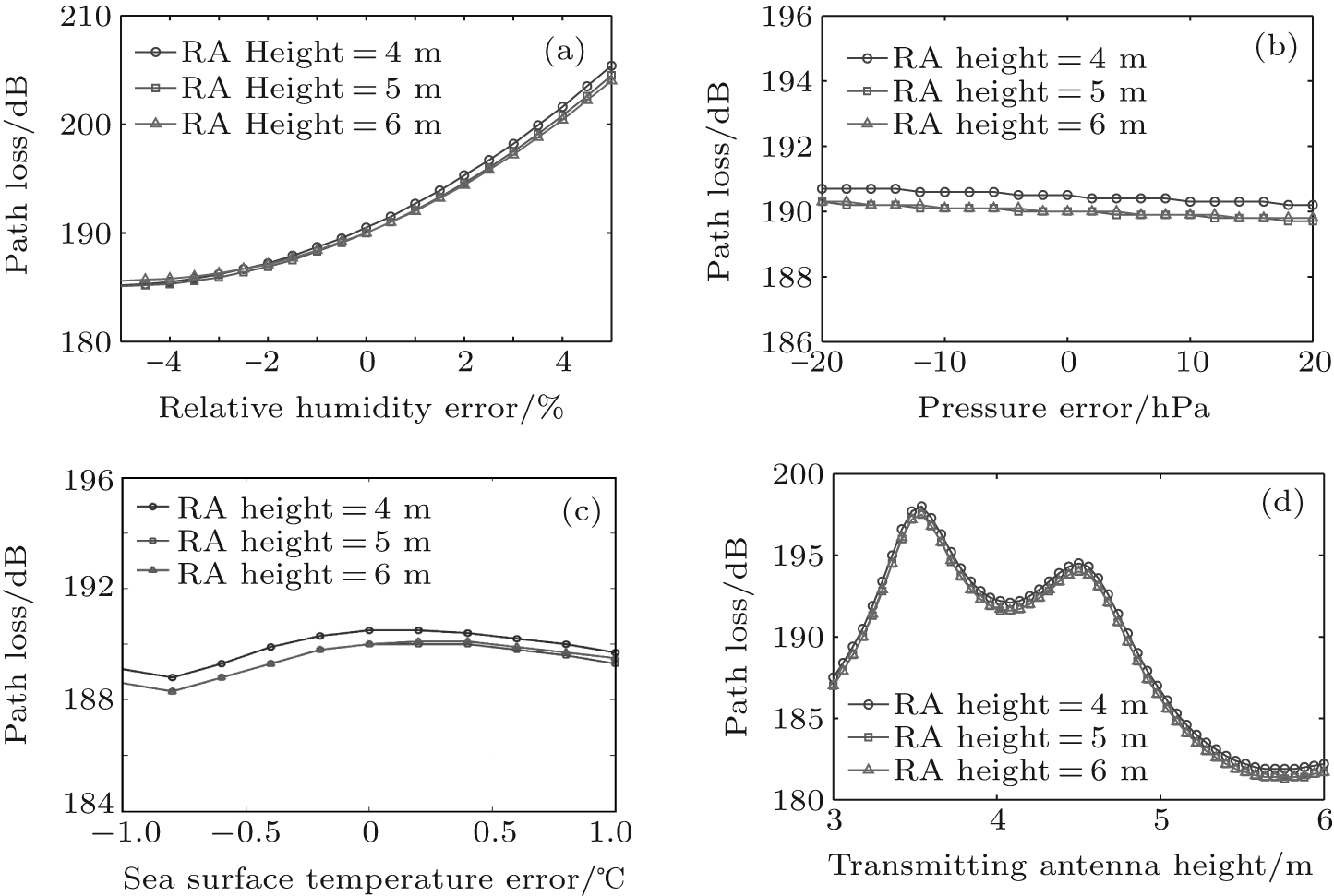 | Fig. 10. (a) The impact of relative humidity error on path loss. (b) The impact of pressure error on the path loss. (c) The impact of sea surface temperature error on path loss. (d) The impact of transmitting antenna height error on the path loss. |
The transmitting antenna height is about 4.5 m and the receiving antenna height is about 5 m in the experiment. However, they may change due to the tide and waves and the accurate antenna height was hard to measure during the experiment. Figure 10(d) shows the impact of antenna height on path loss calculated by the APM model. It shows that if the transmitting antenna height is reduced to 3.5 m, the path loss will increase about 5– 6 dB. Meanwhile, the receiving antenna height has slight influence on the path loss. When the receiving antenna height changes from 4 m to 6 m, the path loss changes only about 1– 2 dB.
In this paper, the influence of obstacle on electromagnetic wave propagation in evaporation duct is investigated. The comparison of the electromagnetic wave propagation in an evaporation duct with and without obstacle is presented. The numerical simulation results show that the obstacle causes a significant increase in path loss on electromagnetic wave propagation. The obstacle has a larger impact on electromagnetic wave propagation of high frequency and in the evaporation duct with high EDH. The experimental result shows that the island causes about 30– 40 dB increase in path loss. The error between model and measurement is discussed and the errors of transmitting antenna height and relative humidity are the possible causes of the discrepancy.
The authors express their appreciations to all the participants in evaporation duct experiments held in 2012.
| 1 |
|
| 2 |
|
| 3 |
|
| 4 |
|
| 5 |
|
| 6 |
|
| 7 |
|
| 8 |
|
| 9 |
|
| 10 |
|
| 11 |
|
| 12 |
|
| 13 |
|
| 14 |
|
| 15 |
|
| 16 |
|
| 17 |
|