

A multiple-relaxation-time lattice Boltzmann method for high-speed compressible flows*
[Li Kai, Zhong Cheng-Wen† ]
]
]
 |


†Corresponding author. E-mail: zhongcw@nwpu.edu.cn
*Project supported by the Innovation Fund for Aerospace Science and Technology of China (Grant No. 2009200066) and the Aeronautical Science Fund of China (Grant No. 20111453012).
This paper presents a coupling compressible model of the lattice Boltzmann method. In this model, the multiple-relaxation-time lattice Boltzmann scheme is used for the evolution of density distribution functions, whereas the modified single-relaxation-time (SRT) lattice Boltzmann scheme is applied for the evolution of potential energy distribution functions. The governing equations are discretized with the third-order Monotone Upwind Schemes for scalar conservation laws finite volume scheme. The choice of relaxation coefficients is discussed simply. Through the numerical simulations, it is found that compressible flows with strong shocks can be well simulated by present model. The numerical results agree well with the reference results and are better than that of the SRT version.
The lattice Boltzmann method (LBM)[1] is a modern approach in computational fluid dynamics. Unlike the traditional method that was based on macroscopic equations, the LBM is based on solving the discrete-velocity Boltzmann equation and macroscopic quantities are obtained by the statistics of distribution functions. The appealing merits of the LBM are a simple algebraic operation, linear convective terms, and easy parallelisation. Because of these advantages, LBM has been successfully applied in many areas of fluid mechanics, such as in microflows, [2– 6] turbulent flows, [7– 10] multiphase flows, [11– 13] blood flows, [14– 16] heat transfer flow, [17– 19] etc.
Continuous efforts have been made to improve the LBM since its inception. Besides the single-relaxation-time (SRT) scheme, which has been routinely used, there are several variations of LBM, including the entropic scheme, [20, 21] the two-relaxation-time (TRT) scheme, [22, 23] and the multiple-relaxation-time (MRT) scheme.[24, 25] It should be mentioned that the MRT scheme has attracted much attention in recent years. It is more suitable than SRT scheme in terms of physical principles, parameter selection, and numerical stability.[25] Moreover, when the transformation matrix and moments of MRT scheme are defined, the formulations of equilibrium distribution functions are fixed.
Generally, the LBM model with two-dimension-nine-velocity (D2Q9) lattice and advection-collision evolution process is called the standard LBM. The standard LBM model can only recover the incompressible Navier– Stokes equations. In 1993, Alexander et al.[26] and Qian[27] proposed the multispeed (MS) approach which is a straightforward extension of standard LBM. The models proposed in Refs. [26] and [27] have several drawbacks, such as nonlinear error terms from macroscopic equations, fixed Prandtl number and specific-heat ratio, and low Mach number limit. Chen et al.[28] eliminated the nonlinear error terms by considering higher-order constraints. To obtain adjustable specific-heat ratio, Yan et al.[29] proposed a multi-speed and multi-energy-level model. Sun, [30– 32] Shi et al., [33] Kataoka and Tsutahara, [34, 35] and Watari[36] devised several models that introduced an extra energy into the definition of total internal energy. In 1998, He et al.[37] proposed the first double-distribution-function (DDF) model. In this model, the DDF is used for the flow field and additional internal energy distribution function is used for the temperature field. The DDF model has adjustability for the Prandtl number and specific-heat ratio. Guo et al.[38] proposed a total energy distribution function to replace the internal energy distribution function. Li et al.[39] introduced circular function into the DDF model and achieved satisfactory simulation results in high Mach number flows. On the basis of previous researches, we[40] proposed a potential energy DDF model which keeps the part of the MS approach. During this period, the finite difference and finite volume method are widely used in LBM to obtain more stable and accurate results.
Because of the advantages compared to the SRT model, MRT LBM models have been successfully applied to compressible flows. Zheng et al.[41] developed an MRT LBM which has an adjustable Prandtl number by modifying the collision term of some moments. Chen et al.[42– 44] transferred the model of Kataoka and Tsutahara from SRT LBM to MRT LBM. In this paper we improved the potential energy DDF model by introducing MRT scheme into the evolution of density distribution functions. The moment space and corresponding transformation matrix are constructed for the D2Q17 lattice. Equilibria of the nonconserved moments are chosen so as to recover the complete compressible Navier– Stokes equations through the Chapman– Enskog analysis. Finally, the capability of this model is compared with previous SRT model through several compressible cases that test its robustness.
The rest of the paper is organized as follows. The compressible model and numerical method are described in Section 2 and Section 3, respectively. Section 4 presents selected numerical simulations including the Colella explosion wave and flows round a circular cylinder. The obtained results are compared with available computational results. The last section is dedicated to the concluding remarks.
The discrete Boltzmann Bhatnagar– Gross– Krook (BGK) equation[45] is

where α = 0, 1, 2, … , N is the discrete velocity direction, fα is the density distribution function, 
To have an adjustable specific-heat ratio and Prandtl number and recover the complete Navier– Stokes equations, the potential energy distribution functions are introduced and the corresponding governing equation is[40]

where 
The macroscopic quantities (density, momentums, and total energy) are calculated by
where b is the number of degrees of freedom (DOF).
The potential energy equilibrium distribution function can be simply obtained by

where D is the number of dimensions.
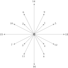
In Ref. [40] the D2Q17 (see Fig. 1) circle function which is proposed by Qu et al.[46] is used. The circular function assumed that all mass, momentum, and energy are concentrated on a circle. The circular function is then distributed amongst the lattice velocities through Lagrangian interpolation with a set of base vectors related to the discrete velocities. The discrete velocities are defined as
 | Fig. 1. D2Q17 discrete velocity model. |
For convenience, the density distribution function space is denoted by f in the following. To construct the MRT model, a moment space m, a N × N transformation matrix M, and a diagonal relaxation matrix S = diag(s0, s1, … , sN) to replace the relaxation coefficient in Eq. (1) are defined. The relationship between the distribution function space and the moment space is

For the D2Q17 model, m is defined specifically as
where density ρ and the momentum (jx, jy) are conserved moments. Other moments are non-conserved moments and their equilibria are functions of the conserved moments in the system. Among them, E is related to the kinetic energy, qx and qy are proportional to the x and y components of the energy flux, and pxx and pxy are proportional to the diagonal and off-diagonal components of the viscous stress tensor.[47, 48]
The matrix M is composed by a set of vectors

where
We find that the same density distribution functions in Refs. [40] and [46] can be obtained when the corresponding equilibria of the moments are defined as
Finally, the governing equations become


where Λ = M− 1SM is the collision matrix.
Through the Chapman– Enskog analysis, the complete compressible Navier– Stokes equations can be recovered when
Other relaxation coefficients are adjustable.
There are two points about the governing equations to be concerned. The first one is that MRT model is not used in Eq. (12). The reason is that it is an additional equation and its only role is to implement the evolution of the potential energy distribution functions. Actually, the result will get worse if the MRT model is used. The second point is that no moment appears in Eq. (11). The moments are just intermediate variables used in the modeling process. This is of benefit because it saves memory during computing.
In standard LBM, the discrete velocities are coupled with configuration space and the evolution is carried out in a fixed way. Hence, standard LBM is hard to be applied on a non-uniform grid. To overcome this problem, many people[49– 52] chose to use finite difference or finite volume methods to solve the discrete Boltzmann BGK equation. Although the increase of complexity goes against the computational efficiency, finite difference or finite volume method makes LBM suitable for non-uniform grid and are also more flexible. There are a wide assortment of numerical schemes to choose from.
In this study, the third-order monotone upwind schemes for scalar conservation laws (MUSCL) finite volume scheme were used.[53, 54] Take the kinetic equation of density distribution function for example, equation (11) can be rewritten as[1, 52]

where 


and n is the outward-directed unit normal vector.
For a two-dimensional structured mesh, the semi-discretized form of Eq. (14) is
where 


where 

where κ = 1/ 3 and s is the van Albada limiter[55]
where ε is a small number to prevent the division by zero error in the region of zero gradient, and
For simplicity, the Euler forward scheme is applied for the temporal discretization. The solution for g follows the same method as f.
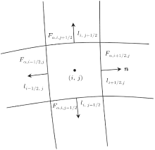
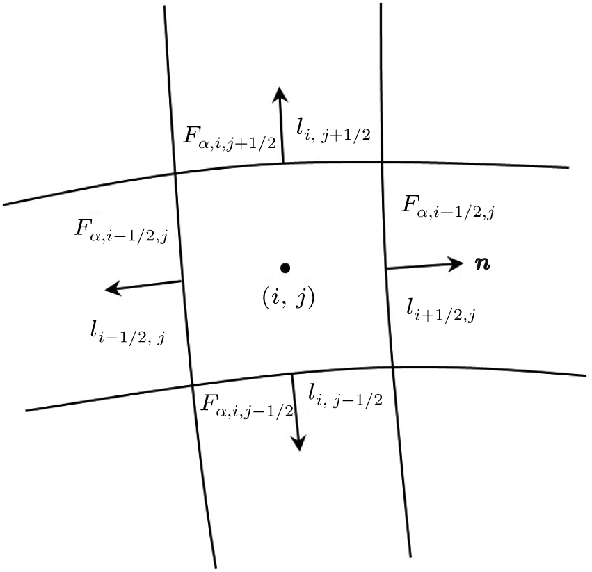 | Fig. 2. Numerical flux on the interfaces of a cell. |
In this section, we conduct a series of numerical simulations to validate the compressible MRT LBM model. The testing problems include Colella explosion wave and flows around a circular cylinder. In present simulations, the characteristic temperature Tc is often set to a value which is a little bit larger than the maximum stagnation temperature in the whole flow field.[39] Throughout this section, the reference density, velocity, temperature, and length are all taken as 1.0.
The Colella explosion wave is a strong temperature discontinuity problem that can be used to study the robustness and precision of numerical methods. As a one-dimensional problem, the size of the grid is Nx × Ny = 401 × 6. The top and bottom boundaries are periodic, and the inlet and outlet are set to the equilibrium. In this part, the specific-heat ratio is γ = 1.4, the Prandtl number is 0.71, and the viscosity is μ = 2 × 10− 5.
The initial condition of the Colella explosion wave is
Subscripts “ L” and “ R” represent macroscopic variables on the left and right sides of the discontinuity. The time step is Δ t = 1 × 10− 5 and the characteristic temperature is Tc = 1000.
There are nine adjustable relaxation coefficients in this MRT model. According to the physical background described in Section 2.2, these adjustable relaxation coefficients can be taken as

In order to measure the error between simulated and analytic results, the normalized mean square errors (NMSE) of density is used
where ρ s is the simulated result, and ρ a is the analytic solution. For the SRT case, NMSEρ = 0.2284.
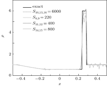
Table 1 shows the values of NMSEρ for some specific values of adjustable relaxation coefficients. It can be seen that the range of the value of adjustable relaxation coefficients which makes the program convergent from 102 to 105 order of magnitude. In this range, NMSEρ first decreases and then increases for all four types of the relaxation coefficients in Eq. (23), and the decrease is faster than the increase. The minimum values of NMSEρ are 0.1782, 0.2035, 0.1775, and 0.2710 for s10, 13, 16, s8, 9, s11, 12, and s14, 15, respectively. The first three values are less than the value of SRT case, but the last one is greater. The corresponding density curves compared with the analytic solution are given in Fig. 3. The fourth curve corresponding to s14, 15 is obviously the worst one. Both the second and third curves have oscillation in the expansion wave and the third curve even has a sharp peak on the left of the shock. Finally, the first one becomes the best choice. So we set s10, 13, 16 to 6000 and the rest relaxation coefficients are equal to sν in the following. In addition, we also find that the optimal value of s10, 13, 16 stays at 6000 when sν changes. This means that the variation of s10, 13, 16 is a general law and can be used in other situations.
| Table 1. The normalized mean square errors (NMSE) of the density. The relaxation coefficients which are not mentioned are equal to sν in each case; × indicates failed calculation. |
 | Fig. 3. Density profiles of Colella explosion wave for different relaxation coefficients at t = 0.012. |
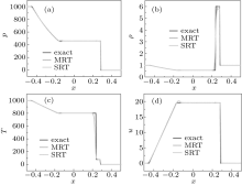
Figure 4 shows the computed pressure, density, temperature, and velocity profiles at t = 0.012, where the SRT results, the MRT results, and the analytical solutions are shown together for comparison purpose. Both the SRT and MRT results capture the shock wave and contact discontinuities well. Because the increasing discontinuity of the initial data immediately spreads out, there is an oscillation of pressure, temperature, and velocity at the right of rarefaction wave. From the density profiles, it can be seen that the MRT results are obviously better than the SRT results. For the pressure, velocity, and temperature, there are no obvious differences.
It is noted that the adjustable relaxation coefficients are analyzed separately. A better result may be found by considering the interaction of relaxation coefficients. However, this is a complex work. The present results have already made a significant improvement.
 | Fig. 4. (a) Pressure, (b) density, (c) temperature, and (d) velocity profiles of Colella explosion wave at t = 0.012. |
In this work, the flows around a circular cylinder are presented at two states. The Mach numbers are 1.7 and 5.0, respectively. The Reynolds number is 2 × 10⁵. The specific-heat ratio is 1.4, and the Prandtl number is 0.71. The H-type grid (see Fig. 5) used in both cases is generated by using the following equation:[56]
where Rx and Ry are the x-direction and y-direction radius of computational domain, respectively, a = tanh (c) with c = 2.5 being a parameter controlling the distribution of the grid. ξ and η are the coordinates of calculation plane.
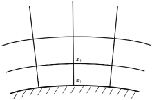
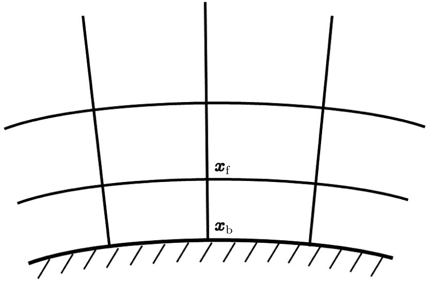
The left inlet is set to the equilibria of the initial condition. At the right outlet, the first-order extrapolation is used for unknown distribution functions. A symmetric boundary condition is applied at the bottom boundary. For the non-slip boundary condition at the surface of the cylinder, the non-equilibrium extrapolation scheme[57] is used. This method is of second-order accuracy. As shown in Fig. 6, xb is a boundary node, and xf is the closest node of xb in fluid field. Then, the distribution function at xb is set to

where the second part in the bracket on the right-hand side is the non-equilibrium part of the distribution function at xf, which is used to approximate the value at node xb.
 | Fig. 5. Grid for supersonic flow past a circular cylinder. |
 | Fig. 6. The diagram of wall boundary. xb is a wall node and xf is the fluid node next to the wall. |
As mentioned before, the variation of adjustable relaxation coefficients is unaffected by the viscosity. Hence, s10, 13, 16 is also set to 6000. Meanwhile, the other relaxation coefficients are equal to sν .
The first case was simulated in Refs. [56] and [58] and can be a reference example to verify the accuracy of the code. In this case, Rx = 4 and Ry = 10, the grid size is 101 × 101, the time step is Δ t = 1 × 10− 5. Figure 7 shows pressure contours in the flow field. We can see that a bow shock is formed in the upstream of the cylinder. The position of the shock is about x = − 3, which agrees with that in Ref. [56]. The reason for the numerical oscillation in the front of the shock is that the grid resolution near the left boundary is coarse.
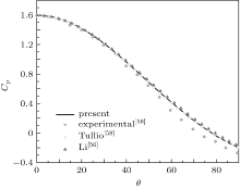
For a more careful examination, figure 8 depicts the pressure coefficient distribution on the surface of the circular cylinder. The pressure coefficients obtained in this study are in a very good agreement with the numerical reference results. The present results are also higher than the experimental results.
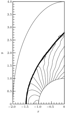
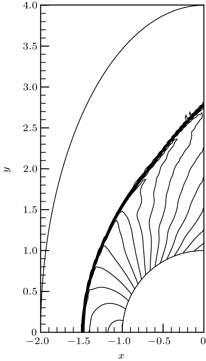
The second case is a high-speed compressible flow. It is predicted that the shock is closer to the circular cylinder. Hence, the computational domain is smaller than that in the first case, Rx = 2 and Ry = 4. The grid size is 151 × 151, and the time step is Δ t = 1 × 10− 6. The pressure contours are shown in Fig. 9. As expected, there is a shock wave at − 1.5 of the x axis. It can be seen that the numerical oscillation in the front of the shock is stronger than preceding case and the
 | Fig. 7. Pressure contours in the vicinity of the circular cylinder at Ma = 1.7. |
 | Fig. 8. Distribution of surface pressure coefficients around the circular cylinder at Ma = 1.7. |
contours have a little deformation near the shock. This means that the present case is close to the limit of the proposed MRT model. The simulation fails when the SRT model is used. It also proves that the MRT model is better than the SRT model.
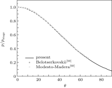
Figure 10 shows the pressure ratio between the local pressure and the static pressure p/ pstag along the circular cylinder surface. The results are in a good agreement with the results from Refs. [59] and [60].
 | Fig. 9. Pressure contours in the vicinity of the circular cylinder at Ma = 5.0. |
 | Fig. 10. Surface pressure distribution around the circular cylinder at Ma = 5.0. |
In this paper, we transpose the potential energy DDF LBM to an MRT model. This model can also recover the complete compressible Navier– Stokes equations with a flexible specific-heat ratio and Prandtl number. With the determination of the equilibria of moments, the same distribution functions with the circle distribution functions are obtained. With the finite volume scheme, numerical experiments include Colella explosion wave and two cases of flow around a circular cylinder are simulated. All of the numerical results obtained from this present approach satisfactorily agree with the analytical solutions or simulation data reported in the available literature. Compared with the SRT model, the present MRT model is more accurate and stable.
| 1 |
|
| 2 |
|
| 3 |
|
| 4 |
|
| 5 |
|
| 6 |
|
| 7 |
|
| 8 |
|
| 9 |
|
| 10 |
|
| 11 |
|
| 12 |
|
| 13 |
|
| 14 |
|
| 15 |
|
| 16 |
|
| 17 |
|
| 18 |
|
| 19 |
|
| 20 |
|
| 21 |
|
| 22 |
|
| 23 |
|
| 24 |
|
| 25 |
|
| 26 |
|
| 27 |
|
| 28 |
|
| 29 |
|
| 30 |
|
| 31 |
|
| 32 |
|
| 33 |
|
| 34 |
|
| 35 |
|
| 36 |
|
| 37 |
|
| 38 |
|
| 39 |
|
| 40 |
|
| 41 |
|
| 42 |
|
| 43 |
|
| 44 |
|
| 45 |
|
| 46 |
|
| 47 |
|
| 48 |
|
| 49 |
|
| 50 |
|
| 51 |
|
| 52 |
|
| 53 |
|
| 54 |
|
| 55 |
|
| 56 |
|
| 57 |
|
| 58 |
|
| 59 |
|
| 60 |
|