

Micro-Gal level gravity measurements with cold atom interferometry*
[Zhou Min-Kang, Duan Xiao-Chun, Chen Le-Le, Luo Qin, Xu Yao-Yao, Hu Zhong-Kun† ]
]
]


†Corresponding author. E-mail: zkhu@hust.edu.cn
*Project supported by the National Natural Science Foundation of China (Grant Nos. 41127002, 11204094, 11205064, and 11474115) and the National High Technology Research and Development Program of China (Grant No. 2011AA060503).
Developments of the micro-Gal level gravimeter based on atom interferometry are reviewed, and the recent progress and results of our group are also presented. Atom interferometric gravimeters have shown high resolution and accuracy for gravity measurements. This kind of quantum sensor has excited world-wide interest for both practical applications and fundamental research.
It is well known that the earth’ s gravitational field is one of the most important environments that human being live in. Gravitational acceleration g, a key parameter of gravity, is time and location dependent. Terrestrial gravity measurements have been performed for more than 200 years with different instruments.[1] Precision measurements of g are of interest in a wide array of applications in geophysics and gravity surveys, [2– 5] fundamental research, [6] natural resource explorations, [7] and other scientific fields.[8] In geophysics, high precision gravity measurements are an important way for acquiring data; for example, the research on geodynamic and tides models.[9] Tests of the post Newtonian gravitational theory, for instance, a kind of standard model extension (SME) theory was figured out by a μ Gal-level (1 μ Gal = 10− 9g and g ≈ 9.8 m/s2) gravimeter.[10] The gravitational constant G was also determined with gravity sensors.[6, 11] Another active motivation to perform gravity measurements is that the gravity mapping has very important applications in natural resource explorations.[12] The gravity and gravity gradient data can be used to reveal underground mass distribution; thus the gravity measurements could offer an efficient way for resource explorations. Accuracy and resolution of g measurements depend on the development of gravimeters. According to the principle, there are two types of gravimeters, relative and absolute gravimeters. Relative gravimeters (RG) are capable of measuring the gravity variations in one site and can compare the gravity value between different sites. RGs usually feature high sensitivity and are widely used in gravity surveys over large areas. Spring type relative gravimeters, [13] relying on a spring– mass accelerometer system, have a noise level of 0.1 μ Gal. The commercial spring gravimeter is either a quartz spring or a zero length spring system, which is compact and suitable for field work. The most sensitive RG is the superconductor one, which has reached a precision of 0.01 μ Gal after one minute integration.[14] A liquid helium cooled diamagnetic superconducting niobium sphere is suspended in an extremely stable magnetic field produced by coils. The electric current of the coils is proportional to the gravity variations. Thus by monitoring the current, the local gravity can be precisely determined.[15] The airborne or satellite gravimeters also belong to the relative type, but are designed to perform global gravity measurements; for instance, the GOCE and GRACE project.[12] Some linear or non-linear output drifts can easily occur in a relative gravimeter, which brings some troubles for long time measurements. Another disadvantage is that the absolute value is unknown when using only a relative gravimeter. Thus a relative gravimeter should be calibrated by an absolute one.
The simple pendulum gravimeter was used in the 19th century by Kater.[16] The value of gravity acceleration is deduced by measuring the period of a pendulum, which is a well-known principle for absolute gravimeters. But the precision is only 10− 5g, as the pendulum is working in a quasi-free mode.[17] With the development of laser and laser interferometry technology, free fall absolute gravimeters have been demonstrated since the 1960s.[18] The test mass during the whole measurement is free falling, and the position of the free-fall test body is recorded by a Michelson interferometer. Then the local gravity is obtained by the fringe counting method. The FG-5 gravimeter is a typical high sensitivity absolute gravimeter.[19] This gravimeter is constructed by a dropping mirror, a laser interferometer, and a compact vibration isolator. FG-5 has reached a sensitivity.[20] of 10 μ Gal/Hz1/2. The accuracy.[19] of this type of gravimeter is about 2– 5 μ Gal, which represents the state-of- the-art level for absolute gravity measurements.
The matter wave interferometer was conceived by Louis de Broglie, who proposed that a photon and a microscopic particle have wave– particle duality. The wave length of a particle is related to its momentum by λ dB = h/p. The diffraction of electrons provided the first matter wave experiments.[21] Compared to photons, the material particle used in a matter wave interferometer is massive, which gives a promising method for inertial sensors. Moreover, particles such as atoms have abundant internal energy levels, which means that it is possible to apply a matter wave interferometer in fundamental research. However, the de Broglie wavelength is very short due to the particle’ s large momentum, it has been a long time since scientists realized matter-wave interferometers with heavy particles because it is difficult to find matched natural gratings, beam splitters, and beam reflectors for particles with the short de Broglie wave length. Since the end of 1970s, huge improvements in technology have been made for controlling and manipulating natural atoms.[22, 23] Especially, the success in laser cooling and trapping natural atoms[24– 30] promised a perfect particle source for scientific research, which induced a revolution in modern physics and led directly to two Nobel prizes.[31– 34] Heavy atoms, such as alkali atoms, can be cooled down to micro Kelvin or even sub-micro Kelvin, so the particle’ s momentum is decreased dramatically, and the de Broglie wave length is then large enough, such that people can coherently manipulate the cooled atoms with laser standing wave-like gratings for beam splitters and reflectors.
Cold atoms have an obvious advantage as the probe for precision measurements, and are the ideal source for matter wave interferometers.[35] The low thermal expansion speed of the cold sample allows people to increase the measurement time. The small first-order Doppler frequency shift permits a longer coherent time when cold atoms are used as the matter wave source. Atom interferometers (AI) have been demonstrated and are involved in fundamental research.[36– 39] The Ramsey type atom interferometers based on the cold atom fountain are used to promise accurate time standards.[40] The Raman type AIs[37] are highly developed and widely used in gravity measurements, [41– 48] gyroscopes, [49– 51] magnetic field sensors, [52, 53] and other applications.[54– 60] Large momentum transfer AIs, [61– 63] such as the Bragg type AI, are employed in the determination of fine structure constants. Trapped AIs in an optical lattice with Bloch oscillations are developed to measure the short range forces between atoms and a surface.[64, 65] Atom interferometers with other new schemes are also proposed to provide high precision measurements.[66– 68]
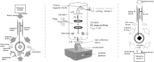
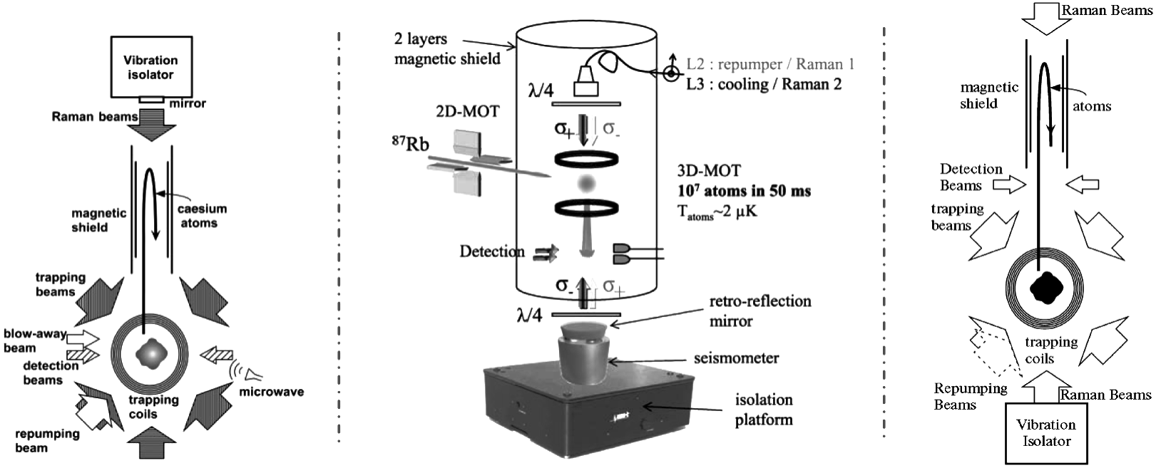
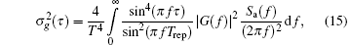
The cold atom interferometry gravimeter has excited worldwide interest.[42, 44, 69– 74] This kind of quantum sensor has the advantage of high potential sensitivity, and is of particular value, there is no mechanical friction between atoms and the vacuum chamber during the recapture of the test mass, which allows performing long time absolute gravity measurements. In addition to the important applications in geophysics and geodesy, high precision atom gravimeters have been proposed to find natural resources, [69] to determine the gravitational constant G, [11, 75, 76] to test the equivalence principle, [77] and to detect gravitational waves.[67] Atom gravimeters will also be useful tools for navigation and gravimetry in space.[47, 55] The first cold atom interferometry gravimeter was demonstrated by Chu et al. in 1991.[37] Sodium atoms were launched and free falling in an atom fountain, and the acceleration of the sodium atoms was measured by an atom interferometry. After several years of improvements, the cesium atom gravimeter[43] of Chu’ s group has reached a sensitivity of 8× 10− 9g/Hz1/2, and an accuracy of several μ Gal. Chu’ s gravimeter is shown in Fig. 1(a); cesium atoms are cooled in a magneto-optical trap and then launched to form an atom fountain. Two-photon stimulated Raman transition pulses are used as beam splitters and reflectors. The wave packet is separated along the vertical direction with a π /2 pulse, then reflected by a π pulse, and finally combined by the last π /2 pulse. The interference pattern is then obtained by measuring the populations of the internal states. The gravity induced phase shift is read out by fitting the fringe pattern. The 87Rb atom gravimeter for the Watt balance project at LNE-SYRTE[20, 44] in Paris (Fig. 1(b)) has reached a sensitivity of 6× 10− 9g/Hz1/2. The cold atoms in the Paris gravimeter are directly released from a MOT. They use a post-correction method for vibration noise rejection. The Paris atom gravimeter is compact and portable. The 87Rb fountain gravimeter of Humboldt University (Fig. 1(c)) has reached a sensitivity of 2× 10− 8g/Hz1/2; this gravimeter was designed to be portable.[70] Now many groups are involved in atom gravimeters.[45, 57, 59, 77]
To measure the absolute gravitational acceleration, our group in Huazhong University of Science and Technology (HUST) started the atom gravimeter project in 2005.[78] As mentioned above, atom gravimeters are suitable for continuous gravity measurements with high precision, thus this kind of gravimeter will open an efficient way for making an absolute gravity standard site. The collision shift of 87Rb is small, and the D2 transition line of 87Rb is known at a relative accuracy of 10− 11, so the 87Rb atom is a good candidate for the test mass in a free-fall sub-micro-Gal gravimeter. Experimentally, cold 87Rb atoms are launched by the moving masses along the vertical direction. After state selection, and when the atoms arrive at the interferometry region, phase-locked Raman lasers are used to coherently manipulate the atomic wave packet to form an interferometer. After carefully suppressing the main noise in our atom gravimeter, an ultra-high sensitive atom gravimeter with a sensitivity of 4.2× 10− 9 g/Hz1/2 has been built in our cave lab.[71, 72] Gravity gradiometers with dual atom interferometers are of interest in gravity surveys and fundamental constant determinations. A dual-fringe locking mode atom gravity gradiometer[48] has been realized with a sensitivity of 670 E/Hz1/2, where 1 E = 10− 10g/m. This gradiometer is intended to be a weak force sensor used for gravitational constant measurements in near future.
Both the atom gravimeter and the free-fall mirror gravimeter (like FG-5) are absolute gravimeters, thus the evaluation of their systematic errors is important for measuring the local gravity. Global absolute gravity measurements are essential for geodynamics and geodesy research, especially for building a worldwide gravity network. The absolute gravity data are collected from many free fall type gravimeters sited in different countries, but each gravimeter has its own systematic error due to the specific design and the unknown gravity gradient. A method that could diminish the uncertainty of individual instruments is to make an international comparison. The international comparisons of absolute gravimeters (ICAG) organized by BIPM have been carried out every four years since 1981. Tens of absolute gravimeters from different manufactures meet together and measure local gravity in one lab during the ICAG. The LNE-SYRTE mobile atom gravimeter joined the ICAG twice — the 8thICAG-2009 at BIPM[79] and the 9th ICAG-2013 in Luxembourg. It is very significant and interesting that the quantum sensor and the classical gravimeter work together and make comparisons, which provides a new way for evaluating the systematic errors of the absolute gravimeters.[80]
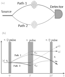
Interferometry plays an important role in modern physics and is mostly used in precision measurements. The wave– particle duality of atoms enables scientists to develop a matter wave interferometer using a well controlled atomic source. Similar to optical interferometers, tools for beam splitting and reflecting are needed to coherently manipulate wave packets in an atom interferometer.[54, 81, 82] Such splitters and reflectors in atom interferometers normally are either mechanically fabricated gratings or laser standing waves. We focus on the two-path atom interferometer, as shown in Fig. 2(a). The phase accumulations of the upper and lower paths are ϕ 1 and ϕ 2, respectively. The phase shift of the interferometry is

Any influence from physical fields that the atom experiences will be included in the phases ϕ 1 and ϕ 2; thus we can use an atom interferometer to perform precision physical measurements, such as measuring the local gravity or an electromagnetic field.
The Raman type atom gravimeter has reached the state-of-the-art level both in sensitivity and accuracy.[72] Low phase noise Raman laser pulses are used as the beam splitter and reflector. Quasi three-level atoms, such as alkali metal atoms, are employed as the matter wave source. Figure 2(b) shows
 | Fig. 2. (a) Schematic of a two-wave atom interferometer. (b) Raman-type atom interferometer, the upper and lower enclosed areas correspond to without and with gravity, respectively. |
the space– time evolution of atom interferometry gravimeters using Raman transitions. We consider 87Rb atoms. There are two stable energy levels in the ground states due to the hyperfine structure. Two far-detuning counter-propagating laser beams in vertical direction couple the ground states and the excited states of the D2 line. The wave vectors of the upper and lower beams are k1 and k2, respectively. The atom is initially prepared in state | a⟩ . The internal state will change to the excited state | i⟩ by absorbing a photon from the upper Raman beam, while the atom’ s momentum increases by ħ k1. After driven by the lower beam, the internal state changes from | i⟩ to | b⟩ through a stimulated radiation, and the atom emits a photon co-propagating with the lower Raman beam. Thus the total momentum change of the atom with this two-photon stimulated Raman transition is ħ (k1 − k2) = ħ keff, while |keff| = |k1| + |k2| ≈ 2|k1|. The internal and external states are coupled together, both of them are transferred coherently after the Raman transition, which means the Raman beam is a good tool for wave packet manipulations to form an atom interferometer.
The physical picture of two-photon stimulated Raman transition is clear; however, we need to know how the internal states population and the phase of the wave-packet evolve during the interaction with the Raman beam. This can be revealed by solving the Schrö dinger equation of the three-level atom and a two-mode laser field system.[81] The electric fields of the Raman beams are
The Hamitonian of this system can be written as

where ω a, ω b, and ω c are the Eigen-frequencies of state | a⟩ , | b⟩ , and | i⟩ , and E = E1 + E2 is the total electric field. In the interaction picture and with the rotating wave approximation, the matrix form of the above Hamitonian is

where Ω ai and Ω bi are the single photon Rabi frequencies, Ω ai = ⟨ a|d · E10|i⟩ /ħ and Ω bi = ⟨ b|d · E20|i⟩ /ħ . The two-photon detuning from the hyperfine structure is

where ω ab = ω a − ω b and ω eff = ω L1 − ω L2. During the evolution, the atom is in a superposition state |Ψ (t)⟩ = ca|a⟩ + cb|b⟩ + ci|i⟩ . Because of the single photon detuning satisfying Δ ≫ δ , the three-level atom can be treated as a two-level atom adiabatically, and the Schrö dinger equation can be simplified as
where ϕ eff = φ 10 − φ 20 is the effective initial Raman phase. The evolution operator of the ground states deduced from the solution of Eq. (5) is

where 
The total phase shift in an atom interferometer is ϕ Total = ϕ E + ϕ L + ϕ S, where ϕ E is the phase shift caused by the atomic wave packet' s free evolution, ϕ L is the phase shift due to the Raman beam, and ϕ S is induced by the nonoverlapping wave packets at the end of the evolution.
The phase shift ϕ E due to the free evolution can be calculated with the path integration method along the two classic paths. The classic action is 
The phase shift ϕ L due to the interaction between atoms and the Raman laser is determined by the evolution operator equation (6). The atomic final state after illuminated by three laser pulses is

where Uπ /2 and Uπ are the evolution operators for π /2 and π pulses. If the atom is in an initial state |a⟩ , by inserting Eq. (6) into Eq. (7), we can obtain the probability of finding atoms in state |b⟩ by

The interference phase due to the Raman laser pulses is ϕ L = 2φ eff2 − φ eff1 − φ eff3, where φ eff1, φ eff2, and φ eff3 are the phases of the three Raman laser pulses. The atoms are free falling during the gravity measurements; thus there must be a huge phase accumulation due to the Doppler shift, which contributes to the interference phase as keff · gT2, where T is the time between neighboring pulses. In order to compensate the Doppler shift to keep resonance, we have to scan the Raman laser frequency linearly. The phase shift induced by frequency scanning is − α T2, where α is the frequency chirp rate. Thus the total interference phase shift of the atom gravimeter is

The earth’ s gravity field is not uniform. We assume that the gravity gradient is γ , and the position, velocity, and gravity at the first Raman pulse are z0, v0, and g0, respectively. The gravity we measured by the atom interferometer is[43]

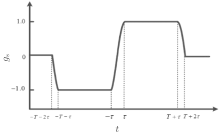
The atom gravimeter is an extremely complex system. Plenty of noise sources can affect the sensitivity of the instrument, such as the Raman laser phase noise, the vibration noise, and so on. The local gravity is obtained by measuring the atomic transition probability P, while all the noise of the gravimeter will cause a fluctuation δ P, and then will affect the interference phase ϕ . The theoretical tool for noise analysis is the sensitivity function.[83] If there is a Raman laser phase disturbance δ ϕ at moment t during the interfering process, the sensitivity function is defined as

The sensitivity function has different formulas at different interference stages. According to the evolution operator equation (6), equation (11) can be detailed as
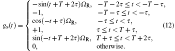
Figure 3 shows that the sensitivity function for a three-pulse Raman type atom interferometer is symmetric.
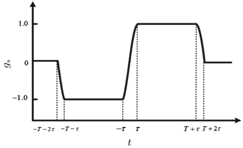 | Fig. 3. The sensitivity function of a three-pulse Raman atom interferometer. |
In the frequency domain, the sensitivity function G(ω ) can be obtained by making a Fourier transformation of gs(t). The transform function H(ω ) of the atom interferometer can be derived via iω G(ω ) as
The noise contribution to the interferometer phase from Raman laser phase noise Sφ (ω ) is
The limit to the resolution of gravity measurements is σ g = σ ϕ /keffT2. Beyond analyzing the effect of the Raman laser phase noise, the sensitivity function is also an efficient tool for evaluating other noise, [44] such as vibration noise, laser intensity fluctuations, and so on.
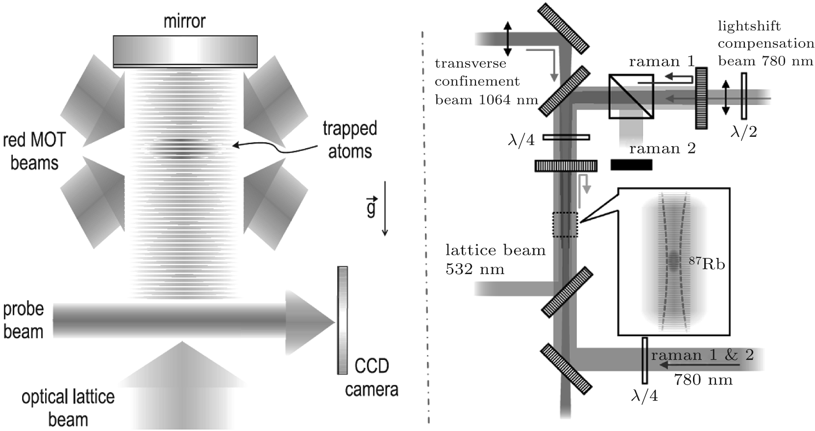
There are two main types of high precision atom gravimeters according to the principle. One is the free fall atom gravimeter using stimulated two-photon Raman transitions, such as the Cs fountain gravimeter at Stanford, the Rb fountain gravimeter at Humboldt University, and the Rb gravimeter with atoms directly released from the MOT at SYRTE. Those free fall gravimeters have μ Gal-level sensitivity. Another type of gravimeter is the trapped atom gravimeter, such as those at SYRTE.[65] and at Firenze University (Fig. 4).[64, 84] The atoms are trapped in an optical lattice, and the gravity is deduced by measuring the tunneling frequency with Bloch oscillations. The sensitivity of the trapped atom gravimeter is lower than that of the free fall gravimeter currently, but it is suitable for measuring short range forces.
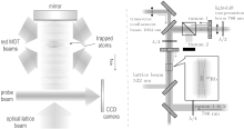
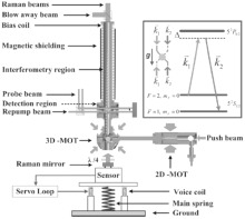
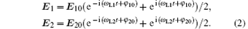
In this review, we will take the atom gravimeter at HUST[71, 72] as an example to give a detailed introduction of making high precision gravity measurements with a quantum sensor. In our experiments, as shown in the inset of Fig. 5, the 87Rb ground hyperfine states with magnetic quantum number mF = 0 are chosen to avoid the first-order Zeeman effect. The ground states | F = 1, mF = 0⟩ and | F = 2, mF = 0⟩ and the excited state | 52P3/2⟩ are treated as a three-level system. In order to measure the gravitational acceleration, the phase-locked Raman beams are oriented in a Doppler-sensitive configuration. When coupled to the counter-propagating Raman beams, the atom in one of the ground states can be excited to the state | 52P3/2⟩ by absorbing the upward (downward) traveling photon, and then the atom will transfer to another ground state after stimulated emission of one photon driven by the downward (upward) traveling Raman beam. The momentum change of the atom is about ħ keff after the two-photon transitions. For a large detuning Δ from the excited states, the three-level atom can be treated as a two-level system. The atom can be coherently driven between the ground hyperfine states by the two-photon Raman transitions to form a Rabi oscillation.
The experimental setup is schematically shown in Fig. 5. The vacuum chamber is made of titanium. In the atom trap stage, a 2D-MOT with a push beam is used to increase the loading rate of the 3D-MOT. When the system is working, the vacuum pressures in the 2D-MOT and the 3D-MOT chambers are about 10− 8 Torr and 10− 10 Torr, respectively. The loading rate of cold atoms in the 3D-MOT can reach about 1× 10¹⁰ atoms/s. In our current experiment, about 3× 10⁹ atoms with a temperature of 7 μ K are trapped within 200 ms. The trapped atoms are then launched with an initial velocity of about 3.83 m/s, corresponding to a flight apex of about 0.75 m relative to the MOT center. After the state preparation, about 5× 10⁷ atoms with a longitudinal temperature of about 300 nK are prepared in the F = 1, mF = 0 state. Afterward, the interference is realized with a π /2– π – π /2 Raman pulse sequence, which is separated by a free evolution time of T. Finally, the populations of atoms in F = 2 and 1 states are detected with the normalized detection method. The whole time used for a single measurement is 1 s.
 | Fig. 5. The experimental setup of an atom gravimeter at HUST.[72] |
The cooling and Raman laser beams used in our experiment are produced by a robust laser system based on two extended cavity diode lasers (ECDL) and two tapered amplifiers. The laser frequency is locked on the transition of | 5S1/2, F = 2⟩ → | 5P3/2, F = 3⟩ by the modulation-transfer stabilized (MTS) method. Then it is amplified to 1 W and shifted about 250 MHz to produce the cooling beams for 2D-MOT and 3D-MOT. The Raman beam is obtained with an optical phase locking loop, and is then shifted by 1.5 GHz with an AOM to form a large detuning from the excited states. The phase noise of the laser beat note in the region of 200 Hz to 200 kHz is less than − 100 dBc/Hz, measured by a phase noise analyzer. The phase noise of low frequencies (less than 100 Hz) is dominant, limited by the 6.834 GHz reference. The Raman beams overlap and are coupled into one single fiber before entering the vacuum chamber, which can reduce the noise accrued in the transferring path. A retroreflector, denoted as the Raman mirror in Fig. 5, is placed under the MOT chamber, which is necessary to realize the counter-propagating configuration by retroreflecting the Raman beams, and there are two pairs of counter-propagating Raman beams in the vertical direction. However, due to the Doppler shift produced by the free falling atoms, only one pair of Raman beams can satisfy the resonant condition by scanning the Raman laser frequency with a rate of 25.14 MHz/s.
As an absolute gravimeter, the resolution of an atom gravimeter is usually limited by vibration noise.[85] As shown in Fig. 5, the Raman beams overlap and enter the vacuum chamber through the top window of the interferometer zone and are reflected by a mirror under the MOT chamber. We can see that most of the critical optical components are common to both beams, except the retroreflecting mirror, and any vertical displacements of the retroreflecting mirror will induce phase noise contributing to the atom interferometer. At present, the mirror is a critical optical component that needs to be well isolated to reduce the dominant noise due to background vibrations. The superspring-type vertical active vibration isolators made by Faller and colleagues were successfully used to improve the measurement precision in corner-cube gravimeters.[86] Active vibration isolators were also used in atom gravimeters.[70, 85]
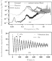
The configuration of the vertical vibration isolator in our atom gravimeter[71] is shown in the bottom of Fig. 5. We use a three-axis commercial seismometer instead of a single-axis accelerometer. The advantage of using a three-dimensional sensor is to obtain the horizontal vibration data, which can be used to analyze the vibration coupling between the vertical and horizontal directions. In the experimental setup shown in Fig. 5, both the accelerometer and the Raman reflector are fixed on a passive vibration isolator. The passive isolator works with a natural resonance frequency of 0.5 Hz, which can isolate the vibration noise above 1 Hz. The output of the accelerometer is digitized and recorded by a 16-bit data acquisition A/D card with a sampling rate of 1 kHz. A loop filter is implemented digitally with the LABVIEW software, which permits us to easily optimize the parameters when the active system is running. The output of the digital loop filter is then used to drive the actuator. We characterize this active isolator by monitoring the acceleration error signal at the output of the sensor. The red circles in Fig. 6(a) represent the typical noise floor of the sensor, which is derived from the data sheet of the seismometer. The other three curves shown in Fig. 6(a) show the equivalent vertical acceleration noise power spectrum density derived from the acceleration error signal. The gray dots indicate the ground vibration noise of our cave laboratory. We can see that the vibration noise below 10 Hz due to seismic motion is lower than 7× 10− 8g/Hz1/2, which means we are already in a very quiet environment compared to a normal experimental site. The gray solid line represents the vibration noise decreased by the passive isolator. The vibration noise around the natural frequency of 0.5 Hz is slightly amplified by the passive isolator, but the vibration noise above 1 Hz is suppressed effectively. The black solid line is the vibration noise of the Raman reflector with the closed feedback loop. The acceleration error signal is greatly reduced by a factor of 100 from 0.1 to 1 Hz. The vibration noise below 2 Hz is less than 1× 10− 9g/Hz1/2, which is probably limited by the intrinsic noise of the sensor and the digitization noise floor of the A/D card. After referring to the active vibration isolator, the limitation of our gravimeter’ s resolution due to vertical vibration noise deduced from the in-loop acceleration signal is less than 1 μ Gal/Hz1/2.
Figure 6(b) shows the step response of the closed-loop system observed from the acceleration error signal. We find that the period Tp is about 63 s by fitting the step response signal; then the natural resonance frequency f0 = 1/Tp = 0.016 Hz. The natural resonance frequency could also be determined from the peak of the black solid curve shown in Fig. 6(a).
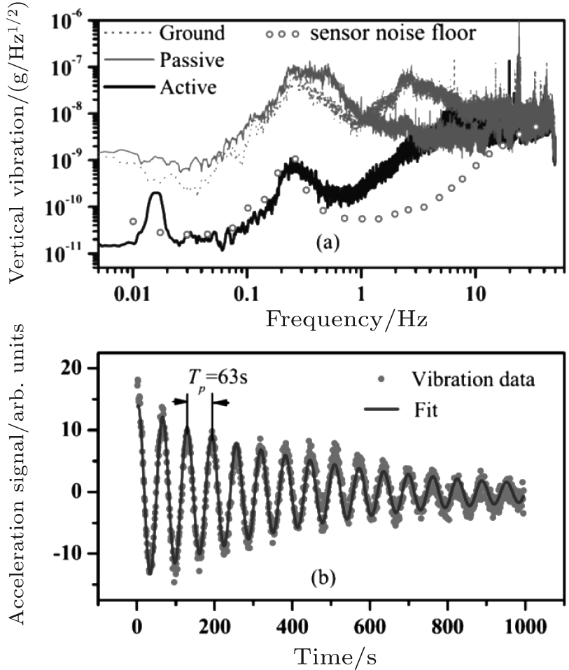 | Fig. 6. (a) Vertical vibration noise of the isolator. (b) Step response of the active vibration isolator.[71] |
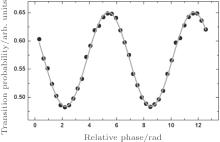
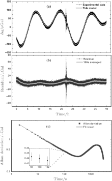
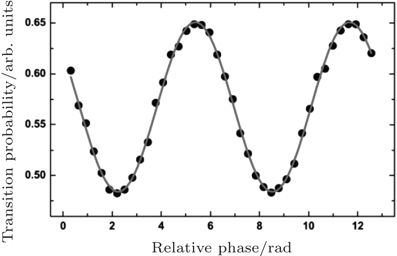
In our experiment, the interference fringe is obtained by slightly changing α with a constant step. Figure 7 shows a typical fringe for a pulse separation time of 300 ms, which contains 40 shots in 40 s. The least-squares sine fitting of the fringe gives an uncertainty of about 11 mrad, which corresponds to a resolution of about 0.8 μ Gal in 40 s. By modulating the central fringe with a phase shift of ± π /2, we can obain an error signal, which is then used to lock the chirp rate of the Raman beam to the fringe center with a digital servo loop.[87] This can be used to give a high-rate gravity measurement on a 2-s interval with a sensitivity better than the method of fringe fitting. In order to evaluate the long-term stability of our gravimeter, a continuous g measurement is carried out for 40 h, as shown in Fig. 8(a). Each point represents two shots in every 2 s. The experimental data are consistent with the theoretical model of the Earth’ s tide. The residual acceleration by subtracting the theory model from the experimental data is
 | Fig. 7. A typical atom-interferometry fringe at a pulse separation of T = 300 ms, the total measuring time is 40 s for 40 shots.[72] |
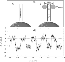
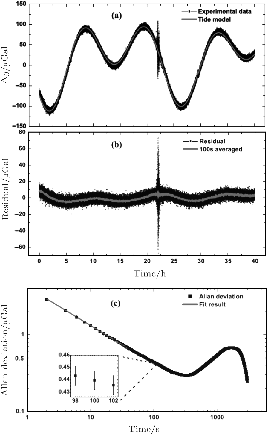 | Fig. 8. Gravity measurements with atom gravimeter.[72] (a) The Earth tides recorded by our gravimeter between 14 and 16 April 2013. (b) The residual tides data by subtracting the theoretical model. (c) Allan deviation of g measurements, showing that the short-term sensitivity has reached 4.2 μ Gal/Hz1/2. |
shown in Fig. 8(b). Seismic waves produced by the earthquake of magnitude 6.6 that occurred in Papua New Guinea on 14 April 2013 are clearly shown in our measurement. The Allan deviation of the gravity measurements is calculated from the residual acceleration, which is shown in Fig. 8(c). The short-term sensitivity up to 100 s given by the Allan deviation is 4.2 μ Gal/Hz1/2. After an integration time of 100 s, the resolution is better than 0.5 μ Gal, as shown in the inset of Fig. 8(c). We have observed a fluctuation of the room temperature in our experiments, which may account for the bump in the Allan deviation at about 2000, as shown in Fig. 8(c). The resolution of this atom gravimeter has been calibrated with additional attracting masses. As shown in Fig. 9(a), two stainless steel SS316 spheres with an individual mass of 8.55 kg are placed around the interferometry region symmetrically and with a vertical distance of 0.045 m above the apex of the atom parabola. The spheres are from the same batch of test masses that were used for measuring G in our cave laboratory.[88] and will produce a theoretical gravitational acceleration shift with an effective mean value of (2.26± 0.07) μ Gal here. By moving the spheres on and off the position with a period of about 40 min, the corresponding acceleration changes can be obtained from the continued gravity acceleration measurement. Figure 9(b) shows the result of the calibration experiment by subtracting the tide effect. Each point is a statistical average of 50 measurements with a time of 100 s, the standard deviation of each point is less than 0.5 μ Gal, which is consistent with the Allan deviation result. The experimental result gives a shift of (2.49± 0.26) μ Gal and agrees with the theoretical calculation. This experiment directly demonstrated that the resolution of our atom gravimeter is better than 0.5 μ Gal with an integration time of 100 s.
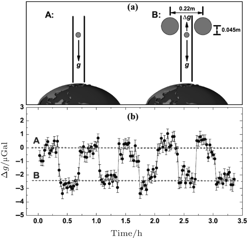 | Fig. 9. Calibrating the resolution of an atom gravimeter with attracting masses.[72] |
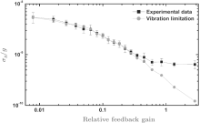
In a high-sensitivity absolute gravimeter, the vertical vibration is usually a dominant noise source as a result of the equivalence principle. Suppressing the residual vibration noise of the Raman mirror is a key issue to achieve such high resolution in our gravimeter. The active vibration isolator used in our gravimeter has been described above. It is capable of changing the level of the residual vibration noise by setting the relative feedback gain between 0 and 3, which is adopted to verify the influence of vibration in our gravimeter. With the vibration noise data obtained from the accelerometer, we can calculate theoretically the limitation due to different vibration noise levels by the equation[44]
where τ is the integration time, Trep is the time for one shot, Sa(f) is the power spectral density of the vibration noise, and G(f) is the Fourier transformation of the sensitive function. The gravity measurements with an integration time of 100 s under different vibration conditions are measured and compared with these theoretical calculations of vibration contribution, which are shown in Fig. 10. We find that the experimental data agree with the theoretical calculation very well when the residual vibration noise dominates. This indicates that the resolution of our gravimeter is no longer limited by the vibration noise at the level of about 0.5 μ Gal in our current experiment, and the resolution limit due to residual vibration noise will be at a level of 0.1 μ Gal with an integration time of 100 s.
 | Fig. 10. Modulation experiments at different vibration noise level.[72] The resolution of the gravimeter (black squares) agrees well with the theoretical calculation of vibration limits (red dots). |
Besides the vertical vibration noise, other noise sources, such as phase noise of the Raman beams and detection noise, also contribute noise to our gravity measurements. For the Raman beams’ phase noise in our gravimeter, the corresponding noise contribution is about 0.8 μ Gal/Hz1/2. To evaluate the contribution of the detection noise, we measure the fluctuation of transition probability versus different atom numbers by changing the loading time. In our current experiment, the loading time is set at 200 ms, and the corresponding standard deviation of transition probability σ p is about 0.0035. This gives a limitation of the resolution as σ g = 2σ p/CkeffT2 per shot, which is about 3.3 μ Gal/Hz1/2, while considering a fringe visibility of about 15% and a pulse separation time of 300 ms. This is mainly induced by the frequency and intensity noise of the probe beam. Further work including robust frequency stabilization and active feedback stabilization of the intensity will be implemented in our future experiment.
Gravity gradiometers have the advantage of rejecting common mode noise, for instance, the vibration noise. Atom-interferometry-based gravity gradiometers have been developed rapidly in recent years.[11, 48, 89] The development of atomic gravity gradiometers has made great progress in gravitational constant measurements with the free fall method. The measurement precision of gravitational constant G is the worst among all the physical constants. There are probably some unknown systematic errors in present measurements. An atom interferometer provides an interesting approach to possible determination of G at the 100 parts-per-million level.
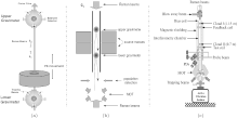
The first atom gradiometer was demonstrated by Kaservich at Stanford.[11, 46, 90] As shown in Fig. 11(a), two MOTs separated by about 1.4 m are employed to launch atoms simultaneously in a vertical direction. The two atom interferometers share one pair of Raman beams. The short-term sensitivity of this gradiometer is 30 E/Hz1/2. Considering the 1.4 m base line, the differential acceleration sensitivity is about 4× 10− 9g/Hz1/2. The atomic gradiometer (Fig. 11(b)) at Firenze group has only one MOT but with a jugging fountain.[89] This gradiometer has a simpler structure. The differential acceleration sensitivity has also reached 3× 10− 9g/Hz1/2. The gravitational constant was measured by this jugging fountain atomic gradiometer at 150 ppm.[76]
 | Fig. 11. (a) The two-MOT atom gradiometer achieved by Mark Kasevich at Stanford.[11] (b) The jugging fountain atom gradiometer at Firenze.[89] (c) The dual-fringe locking atomic gradiometer at HUST; [48] the magnetic field produced by coils is used to make additional feedback. |
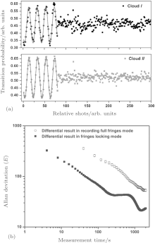
In the conventional operation of atom interferometers based on stimulated Raman transitions, the phase shift induced by Raman lasers is swept to record full interference fringes. However, the measurement data at the extreme points within one full fringe are less sensitive to phase variation than those at the mid-fringe, which will degrade the whole phase measurement sensitivity. In fact, an approach that allows measurements to be invariably performed at the fringe centers has already been adopted for atom gravimeters to improve the sensitivity.[66, 72, 87] In that fringe-locking approach, the Raman laser phase is no longer scanned step by step to sweep one full fringe. Instead, the Raman laser phase is modulated, and then an error is obtained for feedback control of the phase to lock the interferometer at mid-fringe. This real-time feedback ensures that the measurements are always performed at the mid-fringes, regardless of whether there is a change of gravity acceleration or an external disturbance. Atom gravity gradiometers typically consist of two simultaneously operated atom interferometers. It is expected to also be advantageous to operate a gravity gradiometer by the fringe-locking method. However, it is difficult to simultaneously lock two atom interferometers with independent phase shifts at their most sensitive states through the Raman laser phase feedback alone. Here, by introducing an additional feedback control of the magnetic field gradient, we demonstrate an approach that ensures that the two atom interferometers always work simultaneously at the center of their respective fringes by using an additional magnetic feedback.[48] The interference fringes of the upper and lower interferometers, before and after locking, are shown in Fig. 12(a). With this dual-fringe-locking method, the measurement is more sensitive to the gravity gradient signal, and the measurement equations can be linearized at the same time; thus the differential phase shift is directly obtained for every two launches. This measurement approach still retains the intrinsic advantage of rejecting common mode noises, and it is also capable of increasing the sampling rate by about one order of magnitude and improving the sensitivity by about three times in our atom gravity gradiometer, as shown in Fig. 12(b).
This paper has reviewed the history, principles, and experimental realization of atom gravimeters and gradiometers. The sensitivity of atom gravimeters has reached sub-micro-Gal level, which is close to the resolution of cryogenic gravimeters. Atom gravimeters are developing rapidly, and new schemes and technologies are expected to be used. For instance, the large momentum transfer technology with Bragg diffraction or Bloch oscillation could increase the separation between the two interference paths, which would increase the gravity induced phase shift by integer times and hence improve the sensitivity. We expect to employ the Bragg atom interferometry in our atomic gravitational gradiometer, which will enlarge the scale factor by tens of times, and this will help us to improve the uncertainty of measuring the gravitational constant G with free fall atoms. Test of the spin related equivalence principle is also an interesting topic for scientific research. The portable atom gravimeters may also indicate a development trend for gravity instruments. As a high precision quantum sensor, atom interferometry gravimeters give a promising way for ultra-sensitive absolute gravity measurements in geophysics and geodesy. Beyond serving as a sensitive weak-force sensor, atom gravimeters could be useful tools for fundamental research and inertial sensing.
We thank Prof. Luo Jun, Prof. Wang Yuzhu, Prof. Zhou Zebin, Prof. Tu Liangcheng, Prof. Lu Zehuang, Prof. Zhang Jie, Prof. Feng Sheng, and Prof. Liu Xiangdong for enlightening discussions and technical support.
| 1 |
|
| 2 |
|
| 3 |
|
| 4 |
|
| 5 |
|
| 6 |
|
| 7 |
|
| 8 |
|
| 9 |
|
| 10 |
|
| 11 |
|
| 12 |
|
| 13 |
|
| 14 |
|
| 15 |
|
| 16 |
|
| 17 |
|
| 18 |
|
| 19 |
|
| 20 |
|
| 21 |
|
| 22 |
|
| 23 |
|
| 24 |
|
| 25 |
|
| 26 |
|
| 27 |
|
| 28 |
|
| 29 |
|
| 30 |
|
| 31 |
|
| 32 |
|
| 33 |
|
| 34 |
|
| 35 |
|
| 36 |
|
| 37 |
|
| 38 |
|
| 39 |
|
| 40 |
|
| 41 |
|
| 42 |
|
| 43 |
|
| 44 |
|
| 45 |
|
| 46 |
|
| 47 |
|
| 48 |
|
| 49 |
|
| 50 |
|
| 51 |
|
| 52 |
|
| 53 |
|
| 54 |
|
| 55 |
|
| 56 |
|
| 57 |
|
| 58 |
|
| 59 |
|
| 60 |
|
| 61 |
|
| 62 |
|
| 63 |
|
| 64 |
|
| 65 |
|
| 66 |
|
| 67 |
|
| 68 |
|
| 69 |
|
| 70 |
|
| 71 |
|
| 72 |
|
| 73 |
|
| 74 |
|
| 75 |
|
| 76 |
|
| 77 |
|
| 78 |
|
| 79 |
|
| 80 |
|
| 81 |
|
| 82 |
|
| 83 |
|
| 84 |
|
| 85 |
|
| 86 |
|
| 87 |
|
| 88 |
|
| 89 |
|
| 90 |
|