


Understanding many-body physics in one dimension from the Lieb–Liniger model*
[Jiang Yu-Zhua), b) , Chen Yang-Yanga), b) , Guan Xi-Wena), b)†  ]
]
]
|
|


†Corresponding author. E-mail: xwe105@wipm.ac.cn
*Project supported by the National Basic Research Program of China (Grant No. 2012CB922101) and the National Natural Science Foundation of China (Grant Nos. 11374331 and 11304357).
This article presents an elementary introduction on various aspects of the prototypical integrable model the Lieb–Liniger Bose gas ranging from the cooperative to the collective features of many-body phenomena. In 1963, Lieb and Liniger first solved this quantum field theory many-body problem using Bethe’s hypothesis, i.e., a particular form of wavefunction introduced by Bethe in solving the one-dimensional Heisenberg model in 1931. Despite the Lieb–Liniger model is arguably the simplest exactly solvable model, it exhibits rich quantum many-body physics in terms of the aspects of mathematical integrability and physical universality. Moreover, the Yang–Yang grand canonical ensemble description for the model provides us with a deep understanding of quantum statistics, thermodynamics, and quantum critical phenomena at the many-body physical level. Recently, such fundamental physics of this exactly solved model has been attracting growing interest in experiments. Since 2004, there have been more than 20 experimental papers that reported novel observations of different physical aspects of the Lieb–Liniger model in the laboratory. So far the observed results are in excellent agreement with results obtained using the analysis of this simplest exactly solved model. Those experimental observations reveal the unique beauty of integrability.
Mathematical principles play significant roles in understanding quantum physics. The concept “ exact integrability” originally came from the early study of the classical dynamical systems which were described by some differential equations. Usually, the solutions of those differential equations are tantamount to the determination of enough integration constants, i.e., the integrals of motions. In this sense, classical integrability is synonymous with exact solution. However, conceptual understanding of quantum integrability should trace back to Hans Bethe’ s seminal work to obtain the energy eigenstates of the one-dimensional Heisenberg spin chain with the nearest interaction in 1931.[1] He proposed a special form of the wavefunction — superposition of all possible permutations of plane waves in a ring of size L, namely,

where N is the number of down spins and 

The Bethe’ s ansatz appeared to be escaped from physicists’ attention that time. It was only 30 years later that in 1963 Lieb and Liniger[2] first solved the one-dimensional (1D) many-body problem of delta-function interacting bosons by Bethe’ s hypothesis. The exact solution for the delta-function interacting Bose gas was given in terms of the wave numbers ki (i = 1, … , N) satisfying a set of Bethe ansatz equations, called the Lieb– Liniger equations. The spectrum was given by summing up all 

Towards a deeper understanding of the physics of the Lieb– Liniger gas, a significant next step was made by Yang C N and Yang C P on the thermodynamics of this many-body problem in 1969.[3] They for the first time present a grand canonical description of the model in equilibrium. In fact, there are many microscopic states for an equilibrium state of the system at finite temperatures. The minimization of Gibbs free energy gives rise to the so-called Yang– Yang equation that determines the true physical state in an analytical way. In the grand canonical ensemble, the total number of particles can be associated with chemical potential μ . The temperature is associated with the entropy S, counting thermal disorder. This canonical Yang– Yang approach marks a significant step to the exact solutions of finite temperature many-body physics. It shows the subtlety of vacuum fluctuation, interaction effect, excitation modes, criticality, quantum statistics, thermalization, dynamics, correlations, and Luttinger liquid.
The name Bethe’ s hypothesis was coined by Yang C N and Yang C P in the study of the Heisenberg spin chain. The Bethe ansatz is now well accepted as a synonym of quantum integrability. From solving eigenvalue problem of spin-1/2 delta-function interacting Fermi gas, Yang[4] found that the many-body scattering matrix can be reduced to a product of many two-body scattering matrices, i.e., a necessary condition for solvability of the 1D many-body systems. The two-body scattering matrix satisfies a certain intertwined relation, called Yang– Baxter equation. This seminal work has inspired a great deal of developments in physics and mathematics. The Yang– Baxter relation was independently shown by Baxter as the conditions for commuting transfer matrices in two-dimensional statistical mechanics.[5, 6] For such exactly solved models, the energy eigen-spectrum of the model Hamiltonian can be obtained exactly in terms of the Bethe ansatz equations, from which physical properties can be derived via mathematical analysis. The Lieb– Liniger Bose gas[2] and Yang– Gaudin model[4, 7] are both notable Bethe ansatz integrable models.
Yang– Baxter solvable models have flourished into majority in physics since last 70’ s. Later it turned out that the Yang– Baxter integrability plays an important role in physical and mathematical studies.[8– 15] The Bethe ansatz approach has also found success in the realm of condensed matter physics, such as Kondo impurity problems, BCS pairing models, strongly correlated electron systems and spin ladders, cold atoms, quantum optics, quantum statistical mechanics, etc. The Yang– Baxter equation has led to significant developments in mathematics, such as 2D conformal field theory, quantum croups, knot theory, 2D statistical problems, lattice loop models, random walks, etc. Recent research showed that there exists a remarkable connection between conformal field theory and Yang– Baxter integrability of 2D lattice models. Remarkably, conformal field theory has led to the theory of vertex operator algebras, modular tensor categories, and algebraic topology in connection to new states of matter with topological order, such as fractional quantum Hall effect, topological insulators, etc. In this elementary introduction to the exactly solvable Lieb– Liniger model, we will discuss the rigorousness of mathematical integrability and the novelty of quantum many-body effects that comprise the beautiful cold world of many-body systems in the lab. The content of this article involves understanding the fundamental many-body physics through the model of Lieb– Liniger Bose gas.
The paper is organized as follows. In Section 2, we present a rigorous derivation of the Bethe ansatz for the Lieb– Liniger Bose gas. In this section we show how a field theory problem reduces to a quantum-mechanical many-body systems following the Lieb– Liniger’ s derivation. In Section 3, the properties of the ground state are discussed, including ground-state energy, excitations, cooperative and collective features, Luttinger parameter, etc. In Section 4, we introduce the Yang– Yang grand canonical approach to the finite temperature physics of the Lieb– Linger gas. In this section, we demonstrate how the Yang– Yang equation encode the subtle Bose– Einstein statistics, Fermi– Dirac statistics, and Boltzmann statistics. In particular, we give an insightful understanding of quantum criticality. In Section 5, we briefly review some of recent experimental measurements related to the Lieb– Liniger Bose gas from which one can conceive the beauty of the integrability.
We start with introduction of canonical quantum Bose fields 

The Hamiltonian of the 1D single component bosonic quantum gas of N particles in a 1D box with length L is given by[2]

where m is the mass of the bosons, g1D is the coupling constant which is determined by the 1D scattering length g1D = − 2ħ 2/ma1D. The scattering length is given by 
In order to process Lieb and Liniger’ s solution, we first define the vacuum state in the Fock space as 


Considering 

are commutative with the Hamiltonian (1), i.e., [Ĥ , N̂ ] = 0 and [Ĥ , P̂ ] = 0. They are among the conserved quantities of this model. The eigenfunction of the N-particle state | Ψ 〉 for the operators Ĥ , N̂ , and P̂ is given by

where x = {x1, x2, … , xN} and

Here xj is the coordinate position of the j-th particle. For the bosons, the first quantized wavefunction Ψ is symmetric with respect to any exchange of two particles in space x, namely,

In the following discussion, we set ħ = 2m = 1 and c = mg1D/ħ 2. After some algebra, one can find that the eigenvalue problem of the Schrö dinger equation Ĥ | Ψ 〉 = E| Ψ 〉 in N-particle sector reduces to the quantum-mechanical many-body problem which is described by the Schrö dinger equation HΨ (x) = EΨ (x) with the first quantized form of the Hamiltonian
This many-body Hamiltonian describes N bosons with δ -function interaction in one dimension, called the Lieb– Liniger model. This is a physical realistic model in quantum degenerate gases with s-wave scattering potential. In the dilute quantum gases, when the average distance between particles is much larger than the scattering length, the s-wave scattering between two particles at xξ and xη have the following short distance behavior:[19]

where Ψ (x) is the relative wavefunction of the two particles and x is the relative distance between the two particles, i.e., x = xη – xξ . In the above equation, the prime denotes the derivative with respect to x.
In the model (6), the interaction only occurs when two particles contact with each other. Following the Bethe ansatz, [1] we can divide the wavefunction into N! domains according to the positions of the particles Θ (𝒬 ) : x𝒬 1 < x𝒬 2 < … < x𝒬 N, where 𝒬 is the permutation of number set {1, 2, … , N}. The wavefunction can be written as Ψ (x) = ∑ 𝒬 Θ (𝒬 ) ψ 𝒬 (x). Considering the symmetry of bosonic statistics, all the ψ in different domain 𝒬 should be the same, i.e., ψ 𝒬 = ψ 1, where we denote the unitary element of the permutation group as 1 = {1, 2, … , N}. Lieb and Linger wrote the wavefunction for the model (6) as the superposition of N! plane waves[2]

where k’ s are the pseudo-momenta carried by the particles under a periodic boundary condition.
Indeed, after solving Schrö dinger equation HΨ (x) = EΨ (x), we can obtain the same s-wave scattering boundary condition (7) that provides the two-body scattering relation among the coefficients 
where 


When c ≠ 0, all the quasi-momenta are different. If there are two equal pseudo momenta ka = kb, we can prove that the wavefunction ψ 1 = 0.
In general, equation (9) gives the two-body scattering matrix Ŝ , 

then the system is integrable. This relation was independently found by Baxter[5, 6] in studying two-dimensional statistical models. Nowadays, equation (11) is called Yang– Baxter equation. The Yang– Baxter equation guarantees that the multi-body scattering process can be factorized as the product of many two-body scattering processes. This factorization reveals the nature of the integrability, i.e., no diffraction in outgoing waves. For the Lieb– Linger model (6), Ŝ matrix is a scalar function so that the scattering matrix satisfies the Yang– Baxter equation trivially. In the scattering process from 1 to 

With the help of Eq. (12), the eigen wavefunction of the system is given by
Submitting the periodic boundary conditions Ψ (… , xξ = 0, … ) = eiα Ψ (… , xξ = L, … ) into the wavefunction (13), we can find that the pseudo momenta kl satisfies the following Bethe ansatz equations (BAE):
which are called the Lieb– Liniger equations. When α = π , the wavefunction is anti-periodic; while when α = 0, it is periodic. In the following discussion, we only consider the periodic boundary conditions.
Since partial number N̂ and momentum P̂ are conversed quantities of the Lieb– Liniger model, the Hamiltonian together with N̂ and P̂ can be simultaneously diagonalized. For the eigenstate (13), the corresponding particle number 〈 N̂ 〉 = N. For a given set of quasi-momenta {kj}, the total momentum and the energy of the system are obtained as

The solutions to the BAE (14) provide complete spectra of the Lieb– Linger model. The physical solutions to the Bethe ansatz equations require that all the pseudo momenta are distinct to each other. The BAE (14) can be written in the form of phase shift function θ (k) as
where {Ii} are the quantum numbers of pseudo momenta. If N is odd, these quantum numbers are integers, whereas they are half odd integers when N is even. For a given set of quantum numbers {Ii}, there is a unique set of real values {ki} for c > 0. These quantum numbers are independent of coupling constant c. The total momentum can be expressed as
For the ground state, P = 0, where all quasi-momenta {ki} are located in an interval (– Q, Q). Here Q is the cut-off. For the ground state, the quantum numbers are given by

In the thermodynamic limit, i.e., N, L → ∞ and the particle density n = N/L is a constant, the BAE (16) can be written in the integral form

where ρ (k) is the density distribution function of the quasi-momenta defined by the particle numbers in a small interval of (k, k + Δ k), i.e.,

Here the cut-off Q is the “ Fermi point” of the pseudo momenta. It is determined by the particle density 

For the ground state, the energy depends on the dimensionless scale γ = Lc/N. Let us make a scaling transformation

we find the ground-state energy per particle,

with 

with the cut-off condition 
For the ground state, the competition of kinetic energy and interaction energy is represented by the dimensionless coupling strength γ . When γ = 0, the system is free bosons, and all the particles are condensed at the zero momentum state; while if there is a small coupling constant, all the k’ s are distinct. At the limit γ = ∞ , the strong repulsion makes the quasi-momentum distribution the same as the one of the free fermions.
It is very insightful to examine the physics of the model in weak coupling limit. In this case the Bethe ansatz roots comprise the semi-circle law. Gaudin firstly noticed such a kind of distribution, [20] followed by several groups.[21, 22] The Fredholm equation (23) is known as the Love equation for the problem of the circular disk condenser. By using Hutson’ s method, Gaudin found the density distribution function and energy density
This result coincides with the perturbative calculation by using the Bogoliubov method.
This problem can also be solved from the original BAE (14). In the weak coupling limit, i.e., Lc ≪ 1, the quasi-momenta kj are proportional to the square root of c and c/(kj – kl) is a small value. Up to the second order of c, the BAE (14) is expanded as[22]
where 


The solution of this differential equation is a Hermite polynomial and qj is the root of the corresponding polynomial of degree N, i.e., HN(q) = 0. We set the order of qj as qj < qj+ 1, then we have 

where the cut-off 

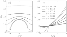
 | Fig. 1. Densities and dressed energies of pseudo momenta for the ground state. (a) Solid lines: the dimensionless densities of the pseudo momenta, ρ ̃ (k) = ρ (k)/c obtained from Eq. (23); dotted lines: the corresponding dimensionless hole densities, ρ ̃ h(k) = ρ h(k)/c. When the coupling strength is small, the distribution function ρ ̃ meets a semi-circle law (27). For the strong coupling limit, i.e., γ ≫ 1, the distribution function gradually becomes flatter and flatter, and approaches ρ (k) ≈ 1/2π . (b) Dimensionless dressed energy is defined by ε ̃ (k) = ε (k)/c3, which is obtained from the dressed energy equation (64). |
In the strong repulsion limit, the gas is known as the Tonks– Girardeau (TG) gas. In realistic experiment with cold atoms, it is practicable to observe the quantum degenerate gas with the strong coupling regime.[23, 24] In the regime γ → ∞ , the Bose– Fermi mapping method[18] can map out the ground-state properties of the Bose gas through the wavefunction of the non-interacting fermions. For finitely strong interaction, γ ≫ 1, we can obtain the ground-state pseudo momenta from the Bethe asnatz equations (14)[25, 26]

where Ij take the ground-state quantum numbers 

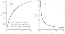
This asymptotic result fits well with the numerical result obtained by solving the integral BAE (19) (see Fig. 2(a)). The ground-state energy (29) can also be obtained from the integral BAE (19) by strong coupling expansion method.[26, 28] We see that for γ → ∞ the leading order of the ground-state energy reduces to that of the free fermions ef = π 2n3/3. One can also calculate other important properties such as compressibility, sound velocity, and Luttinger parameter, once we know the dimensionless function e0(γ ).
Very recently, Ristivojevic obtained high-precision ground-state distribution function for the strong coupling regime[29]

The ground-state energy per unit length and particle density are given by

where λ = (γ + 2)/π − 4π /(3γ 2) + 16π /(3γ 3). The result e0 = E/(Ln3) is plotted in Fig. 2.
 | Fig. 1. The ground state energy and sound velocity for different coupling strength γ . (a) The ground energy density is a monotonic increasing function of γ when the linear density is fixed. Black line: the exact numerical result from Eq. (23). Red line: the weakly coupling expansion result (24). Blue line: the result obtained by the strongly coupling expansion (31). (b) The sound velocity is a monotonic decreasing function of γ . In the weakly coupling limit, the ratio turns to be infinite, while in the strong coupling limit, vs/c → = 2π /γ (see Eq. (45)). |
As discussed in previous section, the eigenstates of the model are described by the quantum numbers {Ij}. We define Ij as a function of the psudomomenta, i.e., I(kj) = Ij, thus we have

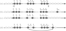
Usually we define the occupied Bethe ansatz roots as particles, while the unoccupied roots as holes. For a hole quasimomentum kh, the quantum number Ih = I(kh) ∈ ℤ + (N + 1)/2. We demonstrate the quantum numbers Ij for the ground state and excited states in Figs. 3(a)– 3(d). For the ground state, there is no hole below the quasi-Fermi momentum, i.e., | k| < Q, whereas the quantum numbers I’ s for the holes site outside the interval [I1, IN] (see Fig. 3(a)).
In the thermodynamic limit, the pseudo momentum distribution function ρ 0(k) for the ground state is determined by Eq. (19) with the cut-off of Q. The ground-state energy and the particle density can be regarded as the function of the cut-off Q, i.e., e(Q) and n(Q). The changes over the configuration of quantum numbers for the ground state give rise to excited states. Figure 3(d) shows such an excitation where the particle with a quasimomentum kh below the pseudo Fermi point is excited outside the Fermi point with a new quasimomentum ke.
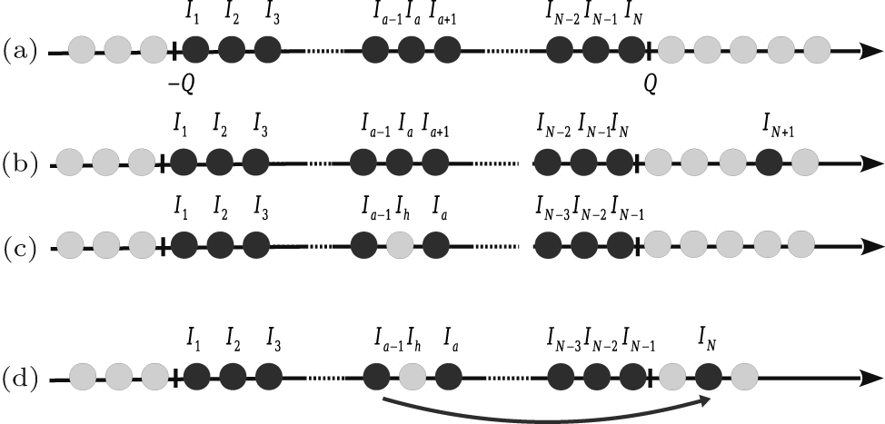 | Fig. 3. Schematic diagrams of the ground state and elementary excitations. (a) Quantum numbers for the ground state. The quantum numbers for the ground state are symmetric around the the origin. The largest quasimomentum denotes the “ Fermi points” ± Q. (b) Configuration of adding a particle near the right Fermi point with the quantum number IN+ 1, so that the total number of particles is N + 1. (c) A hole excitation. The hole at Ih is created so that the total number of particles is N − 1. In panels (b) and (c), the parities of their quantum numbers are changed from half-odd (or integers) to integer (or half-odds) due to the changes of particle numbers. (d) A single particle– hole excitation. A particle at the position Ih is excited out of the pseudo Fermi sea. In this case, the total number of particles is still N, and the parity of quantum numbers dose not change. |
For a single-particle excitation, we decompose the pseudo momentum density into two parts, 


Here we choose a state which satisfies Eq. (19) with cut-off Q as a reference state, i.e.,

The addition of the excited particle leads to a collective rearrangement of the distribution of the pseudo momenta of the N − 1 particles. We denote the difference of the pseudo momentum distribution functions between the excited and the reference state 

The addition of the particle also leads to a shift of the cut-off over the psuado-Fermi point of the ground state of N-particle, i.e., Δ Q = Q – QG. Here, QG is the cut-off for the ground state with the particle number N = LnG(QG), and Q is that for the excited state with 

where μ is the chemical potential, and 

For convenience, we introduce a useful relation between the dressed energy and density. Assuming that two functions f (k) and g (k) satisfy the following equations:
where f0(k) and g0(k) are the driving terms of these integral equations. Then we have the useful relation

By using Eq. (40), from Eqs. (38) and (39), we thus prove that the dressed energy is nothing but the excitation energy of a particle,
On the other hand, the hole excitations impose an additional condition, namely, the maximum momentum is nπ . Similarly, one can prove that the excited energy reads

We plot the dressed energies for different coupling strengths in Fig. 1(b). In order to see clearly excitation spectra, we need to calculate the total momentum using Eq. (17). For both the particle– hole excitation and the Type-II hole excitation, the total particle numbers of particles do not change, as shown in Figs. 3(d) and 4(b). Therefore, the total momenta of the excited states are given by

For the low-energy excitations, ke − Q is a very small value. Therefore, the low-lying behavior can be described by a linear dispersion relation

where vs is the sound velocity of the system. In the above equation, ± corresponds to the excitations at left/right Fermi point, respectively. Nevertheless, for | k| > Q, the relation (44) is the dispersion relation for particle– hole excitations. This linear spectra uniquely determine the universal Luttinger liquid behaviour at the low temperatures. The essential feature resulted from the dispersion relation (44) is such that the system exhibits the conformal invariant in low energy sector. We will further discuss this universal nature of the 1D many-body physics. For the strong coupling, we can obtain the sound velocity from the ground-state energy through the relation 

In Figs. 2(a) and 2(b), we present the analytical and numerical results for the dimensionless energy ē (γ ) = e/n3 and vs/c, respectively.
 | Fig. 4. Dispersion relations in elementary excitations: adding one particle and adding one hole excitation. (a) Solid lines: the spectra for adding one particle to the ground state corresponding to the configuration presented in Fig. 3(b). Dashed lines: the dispersion relations for the hole excitation, see the configuration shown in Fig. 3(c). For γ = 1, the thin blue line is calculated by using Eq. (44). We see that both the particle and hole excitations comprise the dispersion relations with the same velocity. (b) The particle– hole excitation spectra, see Fig. 3(d). The linear dispersion relation is seen for the long-wavelength limit, i.e., the momentum tends to be zero. |
In regard of the strong interacting bosons in 1D, the super Tonks– Girardeau gas is particularly interesting. It describes a gas-like phase of the attractive Bose gas which was first proposed in a system of attractive hard rods by Astrakharchik et al.[30] Batchelor and his coworkers showed its existence of such a novel state in the Lieb– Liniger model with a strong attraction.[31] Due to the large kinetic energy inherited from the repulsive Tonks– Girardeau gas, the hard-core behavior of the particles with Fermi-like pressure prevents the collapse of the super TG phase after the switch of interactions from repulsive to attractive interactions.[32– 35] In fact, the energy can be continuous in the limits c → ± ∞ . From the Bethe ansatz equations (14), near c → ± ∞ , the compressibility is given by
However, for the Lieb– Liniger gas with weak repulsive interaction (0 < c ≪ 1), compressibility is given by

In contrast, the energy for the gas-like phase (super Tonks– Girardeau gas) in weak attractive interaction limit (− 1 ≪ c < 0) is given by

Thus, the compressibility of the super Tonks– Giraread gas with weak attraction is given by

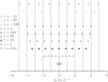
Such different forms of compressibility reveal an important insight into the root patterns of the quasi-momenta. We now show the subtlety of the Bethe ansatz roots for the super Tonks– Girardeau state[32] in Fig. 5.
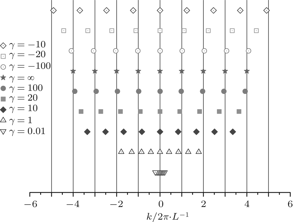 | Fig. 5. Quasi-momenta for the ground state of the Lieb– Liniger gas with the strong repulsion and the supper Tonks– Girardeau gas of the attractive Bose gas for a large value of γ . It is obvious that the super Tons– Girardeau gas has a larger kinetic energy than the free Fermion momentum. Thus the quantum statistics of the super Tonks– Girardeau gas is more exclusive than the free fermion statistics. |
The 1D integrable system gives rise to the power law behavior of long distance or long time asymptotics of correlation functions for the ground state. The effective Hamiltonian can be approximately described by the conformal Hamiltonian which can be written in terms of the generators of the underlying Virasoro algebra with the central charge C = 1. The low-lying excitations present the phonon dispersion Δ E(p) = vsp in the long-wavelength limit. In this limit, all particles participate in the excitations and form a collective motion of bosons which is called the Luttinger liquid.[35] The Lieb– Liniger field theory Hamiltonian can be rewritten as an effective Hamiltonian in long-wavelength limit, which essentially describes the low-energy physics of the Lieb– Linger Bose gas

where the canonical momenta π conjugate to the phase ϕ obeying the standard Bose commutation relations [ϕ (x), π (y)] = iδ (x − y). ∂ xϕ is proportional to the density fluctuations. In this effective Hamiltonian, vs/K fixes the energy for the change of density. In this approach, the density variation in space is viewed as a superposition of harmonic waves.
For example, the leading order of one-particle correlation 〈 ψ † (x)ψ (0)〉 ∼ 1/x1/2K is uniquely determined by the Luttinger parameter K. The Luttinger parameter is defined by the ratio of sound velocity to stiffness, namely,
where vs is the sound velocity and vN is the stiffness and defined as

In Eq. (51), the second expression of the Luttiger parameter is used for numerical calculation with the help of Eq. (22).
Using the asymptotic expansion result of the ground-state energy (24) for weak counting and (29) for the strong counting regimes, we find the asymptotic forms of the Luttinger parameter K for the two limits


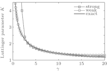
In Fig. 6, we show that these asymptotic forms of the Luttinger parameters provide a very accurate expression throughout the whole parameter space. The correlation functions can be calculated by the conformal field theory.[11, 36– 39]
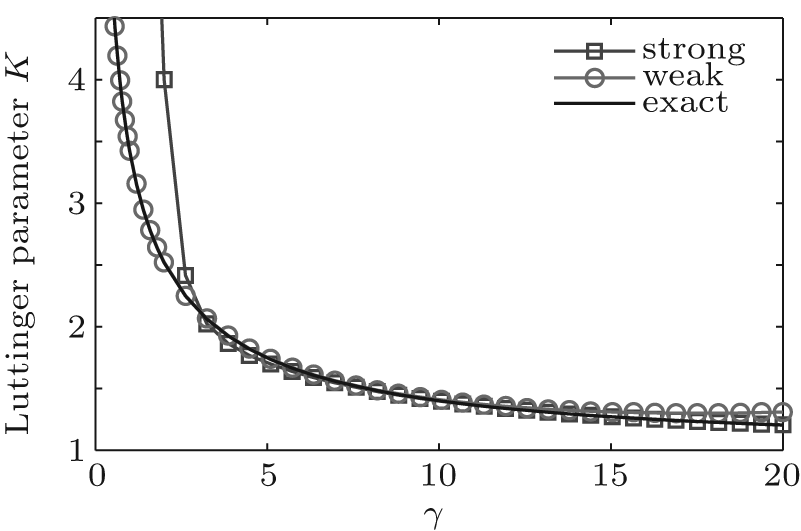 | Fig. 6. Luttinger parameter K versus interaction strength γ . Blue dashed line: the result obtained from Eq. (54) for the strong coupling limit; red dashed line: result obtained from Eq. (53) for weak coupling regime; black solid line: the numerical result obtained from Eq. (51). The analytical result of the Luttinger parameter is in a good agreement with the numerical result. |
Usually, the long-distance or long-time asymptotics of correlation functions of the 1D critical systems can be calculated by using the canonical field theory (CFT).[11] From the CFT, the two-point correlation function for primary fields with the conformal dimensions Δ ± is given by[40]

where τ is the Euclidean time, v is the velocity of light, GO(x, t) = 〈 G| Ô † (x, t)Ô (0, 0)| G〉 is the correlator for the field operators Ô (0, 0) and Ô † (x, t). Equation (55) involves the contributions of the excited states which are characterized by numbers Δ D, N± , and Δ N. Here N− (or N+ ) describes the elementary particle– hole excitations by moving atoms close to the left (or right) pseudo Fermi point outside the Fermi sea with adding N− (or N+ ) holes below the left (or right) Fermi point. Δ N is the change of particle number and it characterizes the elementary excitations by adding (or removing) particles over the ground state. N± and Δ N are not enough to describe all elementary excitations. It is necessary to introduce the quantum number 2Δ D to denote the particle number difference between the right- and left-going particles. From the analysis of finite-size corrections of the BAE, the total momentum and excited energy of the low-lying excitations in terms of these quantum numbers N± , Δ N, and D are given by


where Z = 2π ρ (Q) is the dressed charge at the pseudo Fermi point for the ground state. From the conformal field theory, the excited energy and momentum are given by


By comparison between the two results obtained from finite-size corrections (56), (57), and CFT (58), (59), the conformal dimensions are analytically obtained as a function of N± , Δ N, Δ D, and the dressed charge Z as well, namely,

It turns out that only the low-energy excitations determine the long distance or time asymptotic behavior of the correlation functions. Given that the operator 
We find that the Luttinger parameter K = Z2 by comparing with the result of the Luttinger theory, 
In 1969, Yang C N and Yang C P presented a grand canonical ensemble to describe finite-temperature thermodynamics for the Lieb– Linger model.[3] The Yang– Yang method has led to significant developments in quantum integrable systems.[12, 13, 41] This approach allows one to access full finite temperature physics of the models in terms of the thermodynamic Bethe ansatz (TBA) equations.[12] In the grand canonical ensemble, we usually convert the TBA equations in terms of the dimensionless chemical potential μ ̃ = μ /c2 and the dimensionless temperature T̃ = T/c2 with the interaction strength c. It is also convenient to use the degenerate temperature as an energy unit, i.e., Td = ħ 2n2/2m.[42, 43] It is very insightful to discuss the critical phenomena of the models in terms of the dimensionless units. We first discuss the Yang– Yang grand canonical ensemble below.
For the ground state, the set of quantum numbers (18) provides the lowest energy. However, at finite temperatures, any thermal equilibrium state involves many microscopic eigenstates. As discussed in previous section, these eigenstates are characterized by different quantum numbers {Ij}, see Eq. (16). In the thermodynamic limit, I(k) is a monotonic function of pseudo momenta k.[11] We define dI(k)/(Ldk) = ρ (k) + ρ h(k), where ρ h is the density of the holes. From Eq. (16), we can obtain the integral BAE for arbitrary eigenstate as

Here we should notice that integral interval can extend to the whole real axis, i.e., particles can occupy any real quasimomentum.
In order to understand the equilibrium states of the model, it is essential to introduce the entropy. In a small interval dk, the number of total vacancies is L[ρ (k) + ρ h(k)]dk with a number of Lρ (k)dk particles and a number of Lρ h(k)dk holes. These particles and holes give rise to microscopic states

In the thermodynamic limit, [L(ρ (k) + ρ h(k))dk] ≫ 1 and dk → 0, with the help of Stirling’ s formula, the entropy in this small interval is given by

where η (k) = ρ h(k)/ρ (k). The total entropy is S = ∫ dS. It can be understood from this procedure that the entropy involves the disorder of mixing the particles and holes in the pseudo momentum space. For regions with zero ρ (k) or zero ρ h(k), no disorder occurs, i.e., dS = 0. Therefore, the entropy for the ground state is zero. It is worth noting that the above discussion is valid only in the equilibrium state.
The Gibbs free energy Ω is the thermodynamic potential of grand canonical ensemble for this model,

where μ is the chemical potential, and the particle number is given by N = L ∫ ρ (k) dk. In thermal equilibrium, the true physical state is determined by the conditions of minimizing the Gibbs free energy. Making a virtual change δ ρ , δ ρ h in the thermal equivalent state, we take the variation of the free energy such that

Here we should notice that the variations δ ρ and δ ρ h are not independent in view of the integral BAE (62). This minimization condition leads to the TBA equations in terms of the dressed energy[3]

where the dressed energy is defined by ε (k) = Tln η (k). In the above equation, we also denote ε − (k) = − T ln[1 + e− ε (k)/T]. Using the TBA equation (64), we further obtained the grand thermodynamic potential 

This serves as the equation of state (65) from which we can calculate the thermodynamics of this model at finite temperatures. We can obtain the zero-temperature and finite-temperature phase diagrams of the Lieb– Liniger model. In the zero-temperature limit, the TBA equation (64) reduces to the dressed energy equation (38) in the limit T → 0. From the standard thermodynamic relations, one can calculate the particle density n = ∂ μ p| c, T, entropy density s = ∂ Tp| μ , c, compressibility 

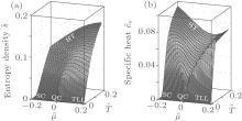
 | Fig. 7. Quantum critical regimes for the Lieb– Liniger model. (a), (b) Dimensionless entropy and specific heat in the T̃ – μ ̃ plane, respectively. For T̃ ≫ 1, it is the HT regime. The TLL with the dynamical exponent z = 2 and correlation length exponent v = 1 lies in the region T̃ ≪ 1 and μ > μ c. For T̃ ≫ | μ − μ c| , the QC regime with z = 2, d = 1, and v = 1/2 fans out near the quantum phase transition point μ ̃ c = 0. It is obvious that the entropy and the specific heat have singularity properties near the critical point μ c = 0. |
In view of the grand canonical ensemble, there exists a quantum phase transition at the chemical potential μ c = 0 at zero temperature. Universal thermodynamics is expected for the temperature under the quantum degenerate regime T ≲ Td, where Td = ħ 2n2/2m.[42, 43] At high temperatures (HT), i.e., T ≫ Td, the system behaves like a classical Boltzmann gas. For μ < μ c = 0 and at low temperatures, the density is very low and the gas becomes de-coherent. This phase is semiclassical (SC). Whereas for μ > μ c and the temperature T < | μ − μ c| , it shows the Tomonaga– Luttinger liquid (TLL) phase. The quantum critical regime lies between SC and TLL for the temperature T ≫ | μ − μ c| . We show such different regimes through the entropy and specific heat in Fig. 7.
Dynamical interaction and thermal fluctuation drive Lieb– Liniger model from one phase into another. In particular, under the degenerate temperature Td, the model has three distinct phases: semi-classical, quantum critical, and the TTL critical phases. At high temperatures, there does not exhibit universal behaviour. When the temperature tends to be infinity, the system reaches the Boltzmann gas. Therefore, the Yang– Yang equation (64) encodes different quantum statistics. For example, when the coupling strength γ → 0, the system behaves as the free bosons; for the strong coupling limit, it behaves like free fermions; at high temperatures, the system becomes the Boltzmann gas. In the following, we rigorously derive such quantum statistics in an analytical way.
When the coupling strength γ turns to be zero, the integral kernel a(k) → δ (x). The dressed energy in this limit can be expressed as

from which we obtain the thermal potential per length 

If γ → ∞ , the dressed energy reads

In this limit, the Bethe ansatz equation (62) naturally reduces to the form

which indicates the Fermi– Dirac statistics. Consequently, the thermal potential per unit length is given by 

We further remark that equations (66)– (70) are valid for arbitrary temperature. If the system is under the quantum degeneracy, the quantum statistical interaction is important. Thus, the particles are indistinguishable. At high temperatures, the Yang– Yang equation (64) gives rise to the Maxwell– Boltzmann statistic such that the particles are distinguishable. In the weak coupling limit and high-temperature limits, it is very convenient to consider Viral expansions with the Yang– Yang equation (64), namely,

Here 
where 
It is remarkable to discover the universal low temperature behavior of the Lieb– Liniger model with the Bose– Einstein statistic and Fermi– Dirac statistic. The Yang– Yang equation (64) provides full physics of the Lieb– Liniger model which goes beyond that can be found by Bose– Fermi mapping.[18] In fact, for strong coupling limit, i.e., γ ≫ 1, the system can be viewed as an ideal gas with the fractional statistics.[43] When the coupling strength is very weak, the ground state behaves like a quasi BEC. The Bogoliubov approach is valid in the weak coupling limit 
In low-energy physics, T ≪ Td, low-lying excitations form a collective motion of bosons. The linear relativistic dispersion near the Fermi points results in the TLL behavior. At finite temperatures, the TLL can be sustained in a region of T < | μ − μ c| in the T– μ plane (see Fig. 7). In the TLL phase, we can take the Sommerfeld expansion with the TBA equation (64). By iterations, the pressure with the leading order temperature correction is given by
which gives the free energy per unit length as the field theory prediction

with the central charge C = 1. Here we took kB = 1, so that in TLL phase the specific heat is linear temperature-dependent

This is a universal signature of the TLL.
However, for the temperature beyond the crossover temperature, i.e., T > T* ∼ | μ − μ c| , the excitations give a non-relativistic dispersion, i.e., Δ E ∼ p2. The crossover temperature T* can be also determined by the breakdown of linear temperature-dependent relation given by Eq. (75).[25] The crossover is also evidenced by the correlation length.[44]
For strong coupling and low temperatures, i.e., γ ≫ 1 and T̃ ≪ 1, the pressure is given by[25]
where 


respectively. Here fn = Lin (− eA/T).
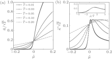
At zero temperature, the quantum phase transition from the vacuum phase into the TLL at the critical point μ c = 0 occurs in the Lieb– Liniger Bose gas. According to the renormalized group theory, universal scaling properties are expected in the critical regime at low temperatures (see Fig. 7). In 2011, Guan and Batchelor investigated the quantum criticality of the Bose gas and found that the equation of state (76) reveals the universal scaling behavior of quantum criticality in terms of the polylogarithm functions.[26] It is straightforward from the equation of the state to derive the universal scaling form of the density as

where the background density n0 = 0. The scaling function 

where κ 0 = 0 and 
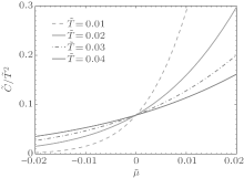
 | Fig. 8. Universal scaling behaviors of the density and compressibility at quantum criticality. (a) Density shows the universal scaling behavior given by (80). (b) Compressibility presents the universal scaling behavior (81). The inset in (b) shows the collapse of temperature-rescaled compressibility  |
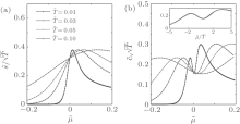
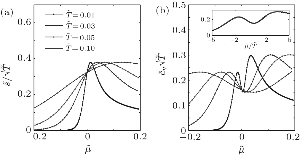 | Fig. 9. Quantum critical behaviour of the entropy and specific heat. (a) The entropy divided by temperature s̃ = s/c has a universal scaling bahavior at the quantum criticality. (b) Specific heat divided by temperature c̃ v = cv/T has a universal scaling bahavior at the quantum criticality. The inset in (b) shows the collapse of  |
Near the critical point, the specific heat divided by the temperature c̃ v ≡ cv/T obeys the following scaling form:
The specific heat at different temperatures has two round peaks near the critical point μ c = 0. These peaks mark the crossover temperatures that distinguish the TLL and semi-classical gas phases from the quantum critical regime. This is a very robust signature for the existence of the crossover temperatures in the 1D Bose gas. This scaling law of the entropy and specific heat is shown in Fig. 9.
In the study of the interacting Bose gas in one dimension, an important property is the local two-body correlation function g2. Physically speaking, this function describes the rates of inelastic collision between pairs of particles.[46– 48] This quantity reflects the probability that the two particles site at the same size. It is also known as contact that strikingly captures the universality of ultracold atoms. This has been described by Tan’ s relations.[49– 51] Tan’ s contact, which measures the two-body correlations at short distances in dilute systems, is a central quantity to ultra-cold atoms. It builds up universal relations among thermodynamic quantities such as the large momentum tail, energy, and dynamic structure factor, through the renowned Tan’ s relations, see recent developments in this research.[52]
Knowing that the two-body correlation can lead to the classification of physically distinct regimes, for example, the Tonks– Girardeau regime with g2 → 0, the Gross– Pitaevskii regime with g2 = 1 and the very weak coupling or fully decoherent regime with g2 = 2. The two-body correlation function can be calculated for these different regimes by expression 


For strong coupling regime, the local pair correlation function is obtained from the equation of state[47, 48, 53, 54]

On the other hand, in one dimension the fundamental thermodynamic relation in a harmonic trap is given by[52]

where ρ s and C are the densities of superfluid and contact, respectively. In this relation, w = vs − vn is the difference between the velocity of the superfluid and normal components. Maxwell relations build the general connections between the contact and other physical quantities such as

Furthermore, we can obtain the contact through the following relations:
The Tan’ s contact of the Lieb– Liniger gas does not have the usual scaling behavior which was found for the interacting Fermi gas in Ref. [52]. This is mainly because the critical field μ c = 0 which does not depend on the scattering length a1D (see Fig. 10).
Over the past few decades, experimental achievements in trapping and cooling ultra-cold atomic gases have revealed beautiful physics of the cold quantum world. In particular, recent breakthrough experiments on trapped ultracold bosonic and fermionic atoms confined to one dimension have provided a precise understanding of significant quantum statistical and strong correlation effects in quantum many-body systems. The particles in the waveguides are tightly confined in two transverse directions and weakly confined in the axial direction. The transverse excitations are fully suppressed by the tight confinements. Thus, the atoms in these waveguides can be effectively characterised by a quasi-1D system. Thus, 1D effective interaction potentials can be controlled in the whole interacting regime by the underlying 3D scattering with tight confinements in the two transverse directions.[16– 18] In such a way, these 1D many-body systems ultimately relate to the integrable models of interacting bosons and fermions. It is now possible to realize effectively one-dimensional quantum Bose gases, in which the interaction strength between ultracold atoms is tunable, see recent reviews.[37, 41] These experiments have successfully demonstrated the anisotropic confinements of atoms to one dimension by optical waveguides, see a feature review article.[55] Particularly striking examples involve the measurements of momentum distribution profiles, [24, 52] the ground state of the Tonks– Girardeau gas, [25] quantum correlations, [56– 61] Yang– Yang thermodynamics, [62, 63] the super Tonks– Girardeau gas, [64] quantum phonon fluctuations, [65– 67] elementary excitations and dark solitons, [68, 69] thermolization and quantum dynamics.[70– 72] More experimental developments of the Lieb– Liniger model are listed in Table 1.[73]
| Table 1. Experiments of Lieb– Liniger gas. |
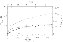
The early experimental studies of the Lieb– Linger gas with cold atoms were made in the laboratory by Bloch’ s group[24] and Weiss’ s group.[25] In particular, the observation of the ground state energy of the Tonks– Girardeau gas provides deep insights into understanding fermionization effect induced by a strong repulsive interaction, see Fig. 11. Loading the 87Rb ultracold atoms into a 2D array of 1D tubes, where the atoms were kept in the lowest energy state in the two transverse directions. Thus, the systems were realized in quasi-1D systems within axial harmonic traps. The essential feature of the Tonks– Girardeau gas was observed through the ground-state energy T1D of such waveguided ensembles.
 | Fig. 11. The 1D ground-state energy T1D versus transverse confinement depth of the lattice. For the confinement potential U0 > 0 (or the effective interaction γ ≫ 1), the energy T1D well presents the ground-state energy of the Lieb– Liniger gas in strong coupling regime within the local density approximation.[16b] |
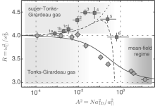
The experimental measurement of the metastable highly excited state — the super Tonks– Girardeau gas was achieved by Haller[64] in 2009. They made a new experimental breakthrough with a stable highly excited gas-like phase in the strongly attractive regime of bosonic Cesium atoms across a confinement-induced resonance, see Fig. 12. This particular state was first predicted theoretically by Astrakharchik et al.[30] Using the Monte Carlo method and by ANU group from the integrable interacting Bose gas with attractive interactions.[31] This model has improved our understanding of quantum statistics and dynamical interaction effect in many-body physics. It turns out that a highly excited state of gas-like gas could be stable as the interaction is switched from strongly repulsive into strongly attractive interactions due to the the existence of Fermi-like pressure.[32– 34] This phenomenon has triggered much attention in theory.[80]
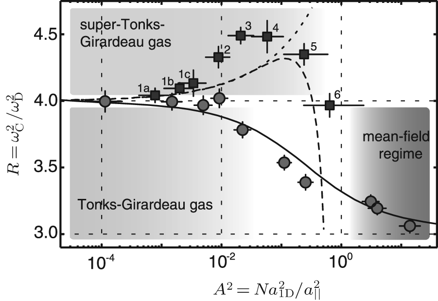 | Fig. 12. The ratio of compress mode over the trapping frequency  |
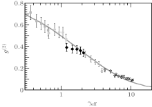
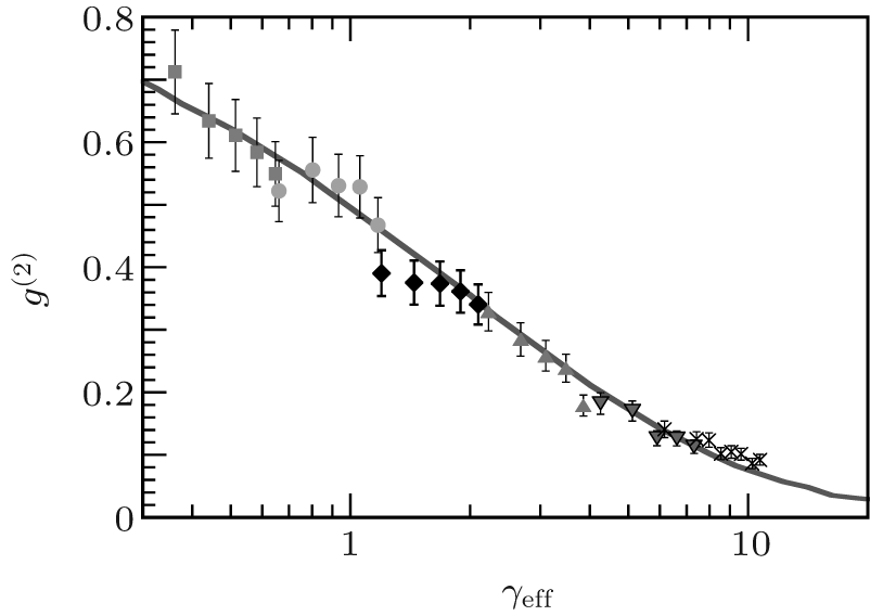 | Fig. 13. The local pair correlation function versus the effective coupling constant. The solid line is obtained from the exactly solved model of Lieb– Linger gas at zero temperature. The symbols show the experimental data.[56] |
In fact, many experiments have successfully demonstrated the confinements of atoms to one dimension by optical waveguides. Another particularly interesting example involves the measurement of photoassociation rates in one-dimensional Bose gases of 87Rb atoms to determine the local pair correlation function g(2)(0) over a range of interaction strengths, see Fig. 13. This experiment provides a direct observation of the fermionization of bosons with increasing interaction strength. It sheds light on the phase coherence behavior.[29, 34, 42, 43, 81] At zero temperature, the local pair correlation is g(2)(0) ∼ 1 for the weakly interacting Bose gas and g(2)(0) → 0 as the system enters into the Tonks– Girardeau regime.
As discussed in previous sections, the finite-temperature problem of the Lieb– Liniger Bose gas was solved by Yang and Yang in 1969.[3] It turns out that the Yang– Yang thermodynamic equation is an elegant way to analytically access the thermodynamics, quantum fluctions, and quantum criticality. The Yang– Yang thermodynamics have been confirmed in the recent experiments through various thermodynamical properties[62, 63] and quantum fluctuations.[65– 67] A typical example is the measurement of the Yang– Yang thermodynamics on the atom chip, see Fig. 14.
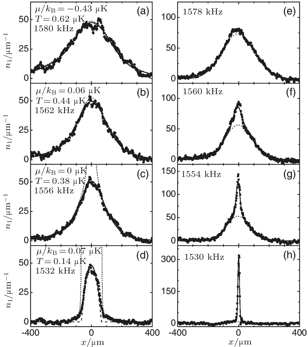 | Fig. 14. The in situ axial density profiles for the weakly interaction Bose gas of 87Rb atoms at different temperatures. The solid lines show the result obtained from the Yang– Yang equations. The values of the chemical potentials are indicated by the harmonically trapping potentials. The experimental data show a good agreement with the theoretical prediction from the Yang– Yang equation.[55] |
Moreover, recent experimental simulations with ultracold atoms provide promising opportunities to test quantum dynamics of many-body systems. In particular, nonequilibrium evolution of an isolated system involves transport and quench dynamics beyond the usual thermal Gibbs mechanism where the ground state and low lying excitation play an essential role. The experimental study[70, 71] of thermalization of 1D ensemble of cold atoms has led to significant developments in this field.[82, 83] In these experiments, it was demonstrated that quenching the dynamics into the isolated systems can lead to non-thermal distributions if conserved laws exist. So far a generalized Gibbs ensemble is believed to present the non-thermal distributions in the isolated systems with conserved laws. The many-body density matrix is written as

in terms of conserved quantities 

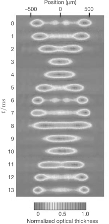
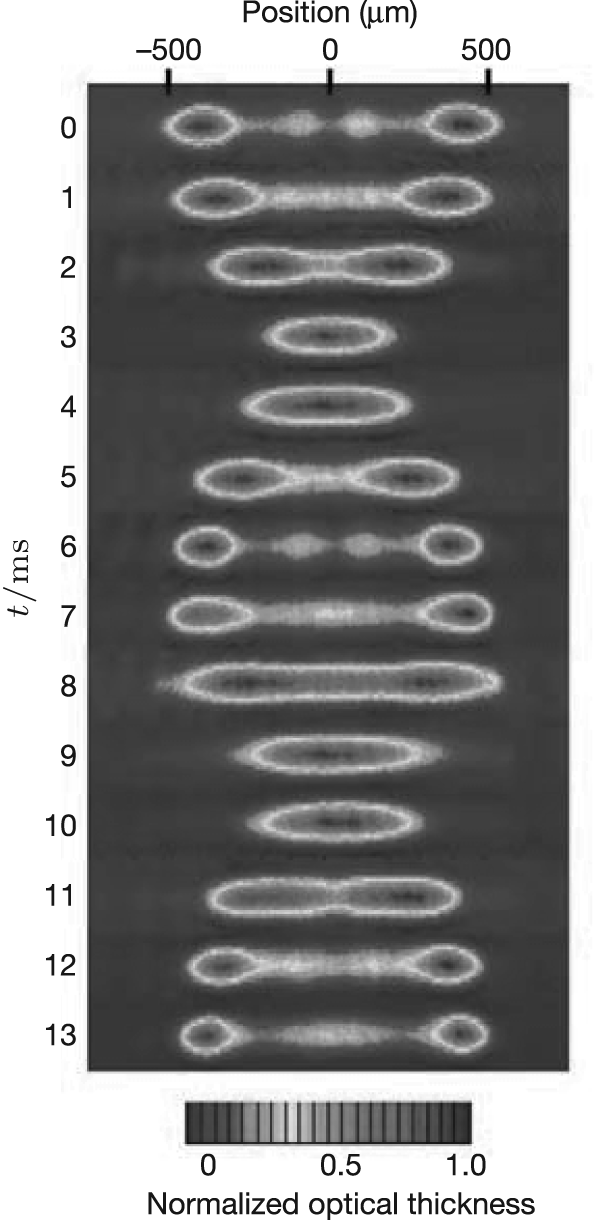 | Fig. 15. The time series of absorption images of the first oscillation cycle for initial average peak coupling strength r0 = 1. The two groups of the cold atoms were confined in one dimension and initially separated by grating pulses. They evolved from time to time and collided twice in the centre of the harmonic 1D trap in each full cycle. The oscillations in 1D Bose gas last for a long time, even without approaching equilibrium.[70] |
Recently, Langen et al.[76] showed that a degenerate 1D Bose gas relaxes to a state that can be described by such a generalized Gibbs ensemble. By splitting a 1D Bose gas into two halves, they prepared a non-equilibrium system of 87Rb atoms trapped in an atomic chip. They measured the local relative phase profile φ (z) between the two halves. It was shown that most of the experimentally reachable initial states evolve in time into the steady states which can be determined within a reasonable precision by far less than N Lagrange multipliers. It was particularly interesting to see that the experimental data of the reduced χ 2 values can be well fitted with about 10 modes although there exist a much larger number of conserved quantities in the system. This research further opens the study of the generalized Gibbs ensemble for the quantum systems out of equilibrium.
We have introduced a fundamental understanding of many-body phenomena in the Lieb– Liniger model. The exact results for various physical properties of the Lieb– Liniger model at T = 0 and at finite temperature were obtained by using the Bethe ansatz equations. In particular, we have presented a precise understanding of the excitation modes, Luttinger liquid, quantum statistics, quantum criticality, correlations, and dynamics in the context of Bethe ansatz. In fact, there have been great developments in the study of the Lieb– Liniger model in Refs. [11, 15, 37] via various methods, such as field theory methods, [34, 84] Luttinger liquid theory and bosonization, etc.[36, 85] It was shown that the repulsive Lieb-Liniger Bose gas can be obtained as the nonrelativistic limit of the sinh-Gordon model.[86– 88] Moreover, the study of the non-thermal distributions for the isolated systems with many conserved laws has attracted much attention. In this scenario, the generalized Gibbs ensemble[83, 89– 92] has been used to study the thermalization of the isolated systems. More recently, there has been growing interest on quench dynamics in terms of the generalized Gibbs Ensemble.[93– 98] This research has been becoming a new frontier in cold atoms and condensed matter physics. It turns out that the integrable systems of this kind thus provide a promising platform to advance the basic understanding of new quantum effects in many-body physics, such as few-body problems, universal thermodynamics, universal contact, quench dynamics, and correlation functions. These studies will further place mathematical theories of exactly solvable models into the laboratory for a wide range of physical phenomena.
This brief introduction to the Bethe ansatz solvable model is based on some informal lectures delivered by the author Guan X W at the University of Science and Technology of China, and Institute for Advanced Study at Tsinghua University.
The author Guan X W thanks Murray T Batchelor, You-Jin Deng, Hui Zhai, Zhen-Sheng Yuan, Fei Zhou, and Qi Zhou for helpful discussion. He acknowledges the Department of Physics, Chinese University of Hong Kong for their kind hospitality.
| 1 |
|
| 2 |
|
| 3 |
|
| 4 |
|
| 5 |
|
| 6 |
|
| 7 |
|
| 8 |
|
| 9 |
|
| 10 |
|
| 11 |
|
| 12 |
|
| 13 |
|
| 14 |
|
| 15 |
|
| 16 |
|
| 17 |
|
| 18 |
|
| 19 |
|
| 20 |
|
| 21 |
|
| 22 |
|
| 23 |
|
| 24 |
|
| 25 |
|
| 26 |
|
| 27 |
|
| 28 |
|
| 29 |
|
| 30 |
|
| 31 |
|
| 32 |
|
| 33 |
|
| 34 |
|
| 35 |
|
| 36 |
|
| 37 |
|
| 38 |
|
| 39 |
|
| 40 |
|
| 41 |
|
| 42 |
|
| 43 |
|
| 44 |
|
| 45 |
|
| 46 |
|
| 47 |
|
| 48 |
|
| 49 |
|
| 50 |
|
| 51 |
|
| 52 |
|
| 53 |
|
| 54 |
|
| 55 |
|
| 56 |
|
| 57 |
|
| 58 |
|
| 59 |
|
| 60 |
|
| 61 |
|
| 62 |
|
| 63 |
|
| 64 |
|
| 65 |
|
| 66 |
|
| 67 |
|
| 68 |
|
| 69 |
|
| 70 |
|
| 71 |
|
| 72 |
|
| 73 |
|
| 74 |
|
| 75 |
|
| 76 |
|
| 77 |
|
| 78 |
|
| 79 |
|
| 80 |
|
| 81 |
|
| 82 |
|
| 83 |
|
| 84 |
|
| 85 |
|
| 86 |
|
| 87 |
|
| 88 |
|
| 89 |
|
| 90 |
|
| 91 |
|
| 92 |
|
| 93 |
|
| 94 |
|
| 95 |
|
| 96 |
|
| 97 |
|
| 98 |
|