Due to the constructive quantum interference along the paths in the discrete or continuous version, quantum walks^{[1, 2]} provided a method to explore all possible paths in a parallel way. Recently, algorithms based on quantum walks have been established as a dominant technique in quantum computation. Up to now, the algorithms based on quantum walks have a great deal of applications, ranging from element distinctness^[3] to database searching, ^{[4– 7]} from constructing quantum Hash schemes^{[8, 9]} to graph isomorphism testing.^{[10, 11]}

There are many kinds of quantum walk models, such as single-particle quantum walks, ^{[12– 15]} two-particle quantum walks, ^{[16– 18]} three-state quantum walks, ^[19] controlled interacting quantum walks, ^{[8, 9]} indistinguishable particle quantum walks, ^{[20, 21]} disordered quantum walk, ^{[22, 23]} etc. Each type of quantum walk has its own special features and advantages.

Lazy quantum walks were presented by Childs to prove that the continuous-time quantum walk is a limit of the discrete-time quantum walk.^[24] He constructed a lazy quantum walk, which only takes one step with a small probability, to obtain small eigenvalues. Hence, the discrete-time quantum walk that reproduces the same properties as those of the continuous-time quantum walk is the appropriate limit. Much attention has been paid to one-dimensional three-state quantum walks recently, ^{[19, 25– 29]} and the limit distribution of these walks has been discussed. In this paper, we will consider the general properties of discrete lazy quantum walks, i.e., three-state quantum walks, such as the order of the moments of the probability distribution, the probability distribution concentrated interval, and the entanglement between the coin and the position of the particle.

Quantum walks have special properties, such as ballistic evolution and high probability of reaching remote points. This is because quantum walks create a superposition of all potential routes, furthermore creating coherent states over these routes. For the Hadamard quantum walks on the line, the probability distribution concentrated interval is .^{[12, 13]} However, previous work has only considered the overall probability distribution concentrated interval, rather than the individual probabilities at the positions in the interval. Therefore, we present the occupancy number and occupancy rate as a measurement of the particle occupancy.

This paper is structured as follows. In Section 2, we introduce the specific mathematical formalism for lazy quantum walks on the line. In Section 3, we study the probability distribution concentrated interval and the moments of the probability distribution for lazy quantum walks, and prove that these moments have the same orders as those for normal quantum walks. We define and analyze the occupancy number and occupancy rate in Section 4 and discuss the entanglement between the position and coin for lazy quantum walks in Section 5. Finally, a short conclusion is given in Section 6.

In general, quantum walks on the line have two directions to move, right and left. But lazy quantum walks have three choices, right, left, and stay put. This results in different behaviour compared to their non-lazy counterparts. In this section, we introduce the specific mathematical formalism for lazy quantum walks on the line.

Lazy quantum walks take place in the product space . is a Hilbert space which has orthonormal basis given by the position states { | x⟩ , x ∈ Ƶ } . The default initial position state is | 0⟩ . Due to the three choices of the movement, lazy quantum walks have a three-dimensional coin. Therefore, is a Hilbert space spanned by the orthonormal basis { | r⟩ , | s⟩ , | l⟩ } (r for right, s for stay put, l for left).

Let | x, α ⟩ be a basis state, where x ∈ Ƶ represents the position of the particle and α ∈ { r, s, l} represents the coin state. The evolution of the whole system at each step of the walk can be described by the global unitary operator, denoted by U,

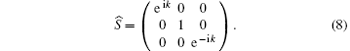
where S is defined as

is the identity matrix which operates in , while C is the coin operation. In this paper, we consider two kinds of coin operators. The first kind is the discrete Fourier transform (DFT) coin operator

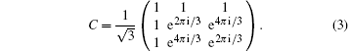
Except for this coin operator, there are other kinds of 3 × 3 coin operators^{[25, 27]}

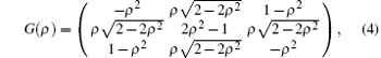
with the coin parameter ρ ∈ (0, 1). This coin operator is equal to the Grover operator when . We will call the parameter ρ the laziness parameter of the lazy quantum walk. Since the position after applying the shifting operator S depends on the coin state of the particle, the walk will generate coin-position entanglement.^[30]

The Fourier analysis is a powerful tool and the right tool to exploit the symmetry of quantum walks. To compare lazy quantum walks with normal quantum walks, in this section, we use Fourier analysis to analytically study the large t behavior of lazy quantum walks.

Firstly, we define the state of the walker, Ψ , at time t ∈ 𝒩 and position x ∈ Ƶ as a three-dimensional vector. We denote this as

Let

with the inverse transform given by

In the momentum space, i.e., the space of , the shift operator becomes

Therefore, the walker evolves following the relation

where Therefore,

It is worth mentioning that 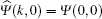. For simplicity, we write as .

As a unitary matrix, has three eigenvalues. If possesses a continuous spectrum and also an isolated eigenvalue, i.e., the eigenvalue is independent of k, the walker will have non-vanishing probability to stay at any position even in the limit of an infinite number of steps.^{[19, 25– 29]}

Next, we will study the large t behavior of lazy quantum walks, specifically the probability distribution concentrated interval and the moments of the probability distribution of the lazy quantum walk.

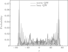
In Fig. 1, we show the probability distributions of the lazy quantum walk and the normal quantum walk. We choose the initial states for lazy/normal quantum walks, respectively, because they can produce symmetrical probability distributions. The choice of the initial state is important in studies of quantum walks, because the interference features sensitively depend on the choice of the coin state. On the other hand, the general properties do not depend on the choice of the initial coin state, so the coin state chosen here is not critical. The coin operators are the DFT matrix and Hadamard matrix. We should note that the 2 × 2 DFT coin operator is precisely the Hadamard matrix, which is the only quantum walk with an unbiased coin operator.^[31] For comparison, we prefer to use the DFT coin operator in this paper.

From Fig. 1, we can see that even though the two kinds of quantum walks have different probability distributions, the probability distribution concentrated intervals for the two quantum walks are close to each other. In Refs. [12] and [13], by using the stationary phase method, the authors reported that for the Hadamard quantum walks, the wave function is almost completely contained in the interval and shrinks quickly outside this region. In Ref. [25], we can also know that the probability distribution concentrated intervals of quantum walks with a coin operator G(ρ ) is [(− ρ + ϵ )t, (ρ + ϵ )t]. Specially, the lazy quantum walk with the Grover coin operator has a probability distribution concentrated interval of .^[19] In short, we conclude that the unbiased normal quantum walk and lazy quantum walks we consider in this paper have the same order of probability distribution concentrated intervals.

Fig. 1.

	Figure Option ViewDownloadNew Window
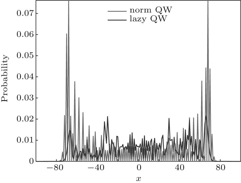	Fig. 1. Probability distribution of the lazy quantum walk and the normal quantum walk. The initial states are and .

Fig. 2.

	Figure Option ViewDownloadNew Window
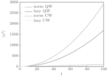
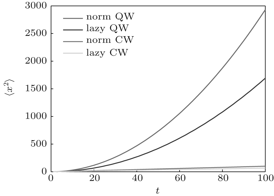	Fig. 2. ⟨ x2⟩ with time t. The initial states for quantum walks are and , respectively.

In Fig. 2 we plot ⟨ x²⟩ for the lazy quantum walk, normal quantum walk, lazy classical walk, and normal classical walk. We still use the states and as the initial states for the two kinds of quantum walks.

From Fig. 2, we see that although the lazy quantum walk has lower values, the values of ⟨ x²⟩ are of the same order of O(t²), which will be proven later. Also, both classical walks have the same order of ⟨ x²⟩ , which is O(t). Furthermore, whether quantum or not, lazy walks have lower values of ⟨ x²⟩ than non-lazy ones. The behavior obviously comes from the lazy action, which stops the walk from going far.

Now we will prove that the probability distributions from lazy quantum walks and normal quantum walks have moments of the same order, defined by

where P(x) is the probability of finding the particle at position x∈ Ƶ .

Theorem 1 The n-th moment of the probability distribution of a t-step lazy quantum walk behaves like O(tⁿ).

Proof Firstly,

Using the relation

where δ (· ) is the Dirac function, we obtain

Since

We now insert Eq. (10) into Eq. (16). Due to the unitarity of U, the eigenvalues of are λ _j = e^{iω _j(k)}, with corresponding eigenvectors of | v_j⟩ (j ∈ { 0, 1, 2} ). Therefore,

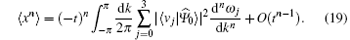
By substituting the eigenvalues and eigenvectors of into Eq. (19), we obtain the value of each moment of the lazy quantum walk. For a quantum walk with coin operator G(ρ ), one of the eigenvalues is 1, which causes the localization effect. For a quantum walk with a DFT coin operator, all eigenvalues of are nonconstant functions of k. Most importantly, all continuous spectrum eigenvalues λ _j^, are functions of e^ik, so dⁿλ _j/ (dkⁿ) ≠ 0, which means dⁿω _j/ (dkⁿ) ≠ 0. Therefore, ⟨ xⁿ⟩ = O(tⁿ). Furthermore, we note that there is no essential difference in the expressions for ⟨ xⁿ⟩ for lazy and normal quantum walks on the line. Hence, the n-th moment of the probability distributions for lazy quantum walks and normal quantum walks are both O(tⁿ).

In Fig. 1, we show the probability distribution of the lazy quantum walk and the normal quantum walk. From the figure, we see that the normal quantum walk has a very high probability of 0.1304 at the position of − 68. While at most positions, the lazy quantum walk has a higher probability. It is worth noting that the normal quantum walk has zero probability at half of the positions in its range. Therefore, normal quantum walks spread quickly, but do not occupy all positions. To measure this aspect of the walks we introduce the concept of occupancy number, always keeping in mind that one number cannot exhibit all properties of a probability distribution.

Firstly, we define the range of a quantum walk.

Definition 1 For a random walk with t steps, the range denoted by N(t) is the number of different positions that the walker could occupy.

In extreme situations, such as when the coin operator is the identity matrix, we note that the range does not change. In fact the range of a quantum walk is only dependent on the shift operator and the number of steps, and is independent of the coin operator and the initial state. For example, a normal quantum walk on the line with t steps has a range of N(t) = 2t + 1. However, a quantum walk whose move choice is to stay or move right has a range of N(t) = t + 1.

Now, we give the definition of occupancy number and occupancy rate.

Definition 2 For a quantum walker walking on a graph, if the walker has a range of N, we define the occupancy number as

where P(x, t) is the probability that the walker is at position x after t steps.

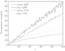
In Fig. 3, we show the dependence of the occupancy number on the number of steps t (the walker‚ s range is 2t + 1). The initial state is still and . It is clear from the graph that the occupancy number of the quantum walks increases linearly with time t, though with fluctuations. This result will be proven later. In addition, the rate of increase for the lazy quantum walks is larger than that for the normal quantum walk. The rate of increase for the lazy classical walk is also larger than that for the normal classical walk. Thus, we see that the lazy action results in a higher occupancy number.

Fig. 3.

	Figure Option ViewDownloadNew Window
	Fig. 3. Occupancy number as a function of time t. The initial states are and , respectively, for two kinds of quantum walks.

The lazy action of the quantum walker brings some new features to the walk. The lazy walker will not have a high probability of being found at a remote position. From another point of view, the lazy walker is more deliberate. The walker does not like to move, and once he moves, he does not like to move again. Hence, the walker has a higher probability (relative to the non-lazy case) of occupying positions that were previously occupied. Furthermore, quantum features, which bring coherence and decoherence, make the walker travel further and give the walker O(tⁿ) order for the moments. In summary, for a lazy quantum walk, the walker has

(i) O(tⁿ) order of the n-th moment;

(ii) a high occupancy number (relative to the non-lazy case);

(iii) similar probability distribution concentrated interval to that of a normal quantum walk.

Because the occupancy number of a quantum walk increases linearly with t, for ease of comparison, we define the occupancy rate as the normalized occupancy number.

Definition 3 For a quantum walker walking on a graph, if the walker has range N, then we define the occupancy rate as

This definition means that the occupancy rate is the quotient of the occupancy number and the range.

In fact, the group-velocity density has the form of

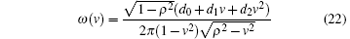
for lazy quantum walks with coin operator G(ρ ), while the normal quantum walks with a general coin operator

has the following density, known as Konno’ s density function

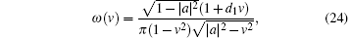
where d₀, d₁, and d₂ are parameters dependent on the coin operator and the initial state. Because

with the group-velocity density, by integrating the group-velocity density on the intervals satisfying P(x, t) ≥ 1/ 2, we can obtain the approximate limit of the occupancy rate. Because the result of the integration is a constant number, OccRate has the order of O(1). OccRate(N, t) has the following properties:

For example, after fifty steps, the occupancy number for the lazy quantum walk in Fig. 3 is 40, while the range is 2(50) + 1 = 101. Therefore, the occupancy rate for the quantum walk after fifty steps is 40/101 ≈ 0.396.

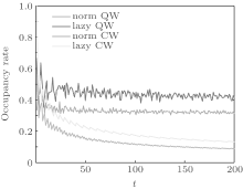
In Fig. 4, we show the dependence of the occupancy rate on the time t. For quantum walks, since the occupancy number increases linearly with t, the occupancy rate is O(1). Also, from Fig. 4, it is clear that the occupancy rate of the quantum walk fluctuates around a fixed value. In general, lazy quantum walks have a higher occupancy rate than other corresponding normal quantum walks on the line, and this behavior also holds for the occupancy number. This is because that for time t, all occupancy rates are the quotients of the respective occupancy numbers and the quantity (2t + 1). Thus, the features of the occupancy rate are the same as those of the occupancy number, except that the order becomes O(1). We should remind readers that the occupancy rate of a classical walk decreases asymptotically to 0 (see Appendix A).

Fig. 4.

	Figure Option ViewDownloadNew Window
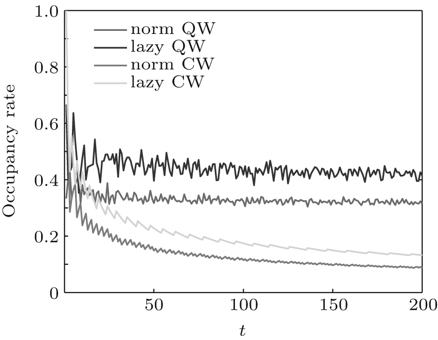	Fig. 4. Occupancy rate versus time t. The initial states are and , respectively, for lazy quantum walks and normal quantum walks.

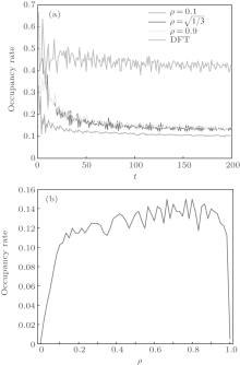
We pose a further question: Do quantum walks with different coin operators all have a high occupancy rate?

In Fig. 5, we plot the occupancy rate versus the time t. In Fig. 5(a), we choose the matrix G in Eq. (4) (with ) and the DFT matrix as the coin operators. In Fig. 5(b), we show the change of occupancy rate at time 200 with laziness ρ . We find that the occupancy rate will increase slowly with varying laziness parameter ρ except a small region near ρ = 0 or 1. Because we choose the occupancy rate at time 200, the occupancy rate in Fig. 5(b) is fluctuant. We also find that, even though the occupancy rate varies with ρ , the maximum value of the occupancy rate for this kind of lazy quantum walk is less than 0.2, which is lower than that for the quantum walk with the DFT coin operator. We also note that the quantum walk with the coin operator has a lower occupancy rate than that for the Hadamard quantum walk. Does this mean that a higher occupancy rate is not a general property of lazy quantum walks? We remind readers that the coin operator G comes from the Grover coin operator, and the corresponding 2 × 2 Grover matrix is the Pauli X matrix, whose occupancy rate is close to 0.

Fig. 5.

	Figure Option ViewDownloadNew Window
	Fig. 5. (a) Occupancy rate versus time t. The initial states are and , respectively, for lazy and non-lazy quantum walks. (b) Occupancy rate versus laziness ρ at time 200.

In more general scenarios, we may want to parameterize the threshold probability, beyond which a position is said to be “ occupied” . Hence, borrowing ideas from the fuzzy set theory, we define the general occupancy number and general occupancy rate using a parameter δ which satisfies 0 < δ ≤ N.

Definition 4 For a quantum walker walking in one dimension, if the walker has range N, then we define the general occupancy number as

Definition 5 For a quantum walker walking in one dimension, if the walker has range N, then we define the general occupancy rate as

The general occupancy rate has the following properties:

GenOccRate(δ ₁, N, t) ≥ GenOccRate(δ ₂, N, t).

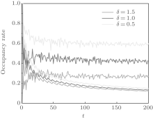
In Fig. 6, we show the general occupancy rate of quantum walks and classical walks for different values of the parameter δ . Blue lines represent the general occupancy rates for quantum walks and classical walks with δ = 1, i.e., the occupancy rates previously considered in Fig. 4. From Fig. 6, we see that the properties of the general occupancy rate do not change with the parameter δ . For quantum walks, the general occupancy rate still converges, with small fluctuations, to a non-zero value, while for classical walks it decreases asymptotically to 0. In addition, the lazy classical walks and normal classical walks have identical orders for their occupancy rates, and the general occupancy rate for both quantum walks and classical walks is O(t). We show in Appendix A that for

Fig. 6.

	Figure Option ViewDownloadNew Window
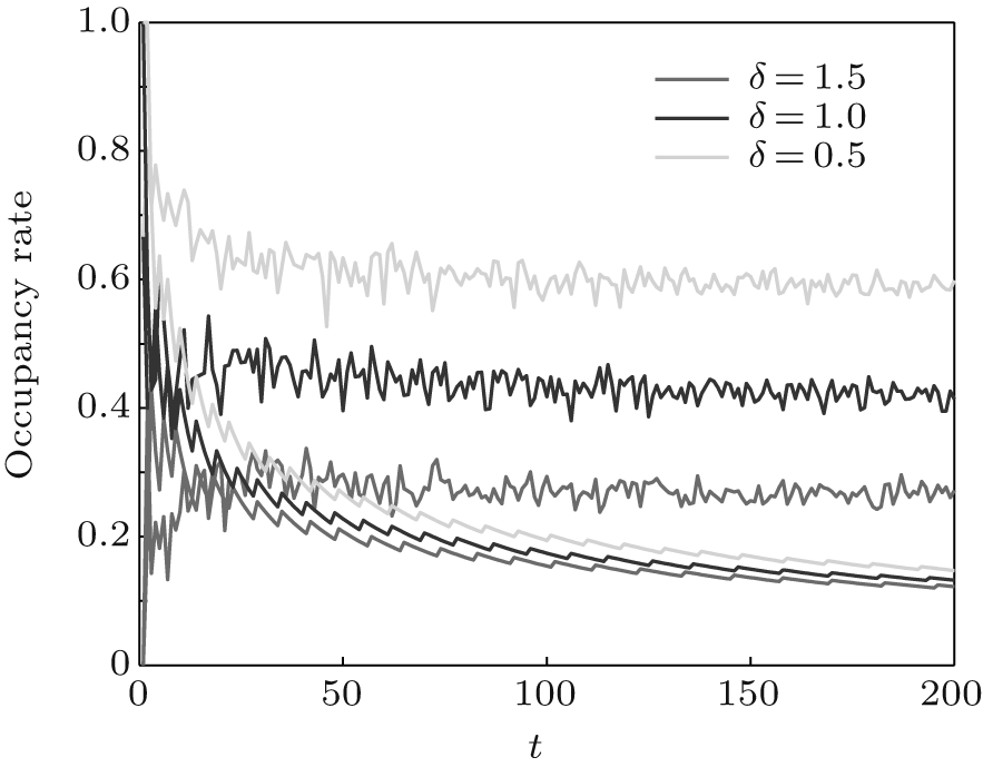	Fig. 6. Dependence of the general occupancy rate on the time t for a 200-step walk. Red lines represent the lazy quantum walk and lazy classical walk with δ = 1.5. Blue lines represent the lazy quantum walk and lazy classical walk with δ = 1. Green lines represent the lazy quantum walk and lazy classical walk with δ = 0.5.

normal classical walks, the occupancy rate is . Therefore, the general occupancy rate for classical walks is also . Furthermore, the general occupancy rate is larger if δ is smaller for all kinds of walks.

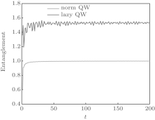
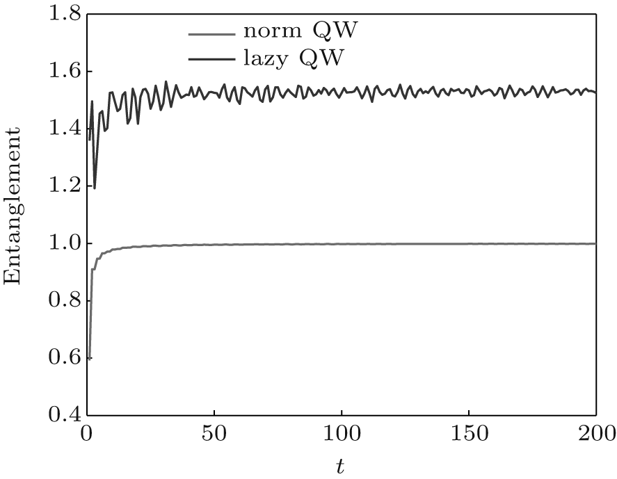
Entanglement is believed to be the most important quantum resource, occurring only in quantum states. For a single particle quantum walk, the entanglement between position and coin is not negligible.^{[32, 33]} In this section, we study the entanglement between position and coin for lazy quantum walks on the line. We use the standard entanglement measure (von Neumann entropy) to measure the total entanglement between the two subsystems: position space and coin space.

The entanglement between the two subsystems of a bipartite pure quantum state | Ψ ⟩ can be quantified using the von Neumann entropy S of the reduced density matrix of either subsystem,

where ρ ₁ and ρ ₂ are, respectively, the reduced density matrices of systems 1 and 2, and 0 log₂ = 0.

Fig. 7.

	Figure Option ViewDownloadNew Window
	Fig. 7. Dependence of ⟨ x2⟩ on time t. The initial states are and for lazy and normal quantum walks, respectively.

Numerical methods can then be used to calculate the entanglement E between position and coin. In Fig. 7, we show the entanglement for normal quantum walks and lazy quantum walks. The maximum value of the entanglement E between two subsystems is E_max = log₂(min(d₁, d₂)), where d₁ and d₂ are the dimensions of the two subsystems. For normal single-particle quantum walks on the line, E_max = log₂(2) = 1, while for lazy single-particle quantum walks on the line E_max = log₂(3) ≈ 1.585. From Fig. 7, we see that the entanglement converges to the maximum value for the two kinds of quantum walks. Because the dimension of the coin space for lazy quantum walks is greater than that for normal quantum walks, the lazy quantum walks have a higher entanglement between position and coin. Although a higher entanglement is a quantum resource, it is achieved at the cost of constructing a three-dimensional coin.

In this paper, we study the properties of discrete lazy quantum walks. We discuss the probability distribution concentrated interval and the moments of lazy quantum walks. We prove that lazy quantum walks and normal quantum walks have the same order for the moments of their probability distributions, O(tⁿ).

We introduce the occupancy number and occupancy rate to measure the extent to which the walk has a relatively high probability at every position in its range. From our study, we conclude that the lazy quantum walks have a higher occupancy rate than other walks such as normal quantum walks, classical walks, and lazy classical walks. We show that the DFT lazy quantum walks and Hadamard quantum walks have similar probability distribution concentrated intervals, but different dissimilar occupancy rates. We also discuss other coin operators. Among the coin operators we consider, the quantum walks with a DFT coin operator have the highest occupancy rate.

Finally, we study the entanglement between position and coin for lazy quantum walks. The entanglement for lazy quantum walks is higher than that for normal quantum walks, which benefits from the higher dimensional coin.

Based on the these properties of lazy quantum walks, we hope in future to find applications.