The Klein– Gordon– Schrö dinger (KGS) equations

describe the interaction between conservative complex neutron field and neutral meson Yukawa in quantum field theory, where ψ (x, t) represents a complex scalar nucleon field, ϕ (x, t) is a real scalar meson field, and . With initial and periodic conditions

there exist a charge conservation law

and a global energy conservation law (GECL)

Massive works^{[1– 3]} with respect to mathematical and theoretical analyses of the KGS equations have been done in the past decades. Studying its numerical approximation has recently become a hot topic. Zhang^[4] derived a charge- and energy-preserving finite difference (C-C) scheme for the KGS equations. During the last decade, many researchers have paid attention to geometrical numerical integrators. Kong et al.^[5] noted that the KGS equations have a multi-symplectic structure and then investigated the multi-symplectic midpoint (M-M) scheme. The explicit multi-symplectic schemes were proposed in Refs. [6] and [7]; while the implicit symplectic Fourier pseudo-spectral schemes were given in Refs. [8] and [6]. Hong et al.^[9] also proposed three schemes, which are called M-C, T-C, and T-T schemes, for the KGS equations. Some other methods can be found in Refs. [10]– [14].

As is well known, the GECL (4) depends on the boundary conditions, such as periodic or homogeneous boundary conditions. However, in practice, the complex boundary conditions lead to the invalidity of the traditional GECL algorithms. Actually, there exists a local energy conservation law, which is more essential than the global energy conservation law. Let ψ (x, t) = p(x, t) + iq(x, t), where p(x, t) and q(x, t) are real-valued functions. By further introducing some variables, the KGS system (1) can be reformed into a combination of ordinary differential equations (ODEs)

Proposition 1 The system (5) possesses a local energy conservation law (LECL)

Proof In Eq. (5a), multiplying the first and the second lines by p_t and q_t, respectively, we have

Next, multiplying the first line of Eq. (5b) by ϕ _t gives

Adding Eqs. (7) and (8) leads to the LECL (6).

The LECL (6) is a local property. In other words, it is independent of the boundary conditions. Thus, the LECL is more essential than the GECL in physics. Naturally, when constructing algorithms for system (5), we expect that the LECL can still hold. Hereafter, we call these numerical methods the local energy-preserving (LEP) algorithms. For the concept of LEP algorithm and its applications, please refer to Refs. [15]– [18]. The aim of this paper is to construct a LEP algorithm for the KGS equations, and then analyze its convergence. Finally, we will check the performance of the proposed scheme.

As usual, we introduce some notations: x_j = a + (j – 1)h, j = 1, 2, … , N + 1; t_k = kτ , k = 0, 1, 2, … K, where h = (b – a)/N and τ are the spatial length and the temporal step span, respectively. Let be an approximation of u(x_j, t_k). We also define the vector 2-norm . To derive the algorithms conveniently, the following operators are used: the finite difference operators ; the averaging operators , ; and the operators , ∀ 0 ≤ a ≤ 1. Especially, we have

Taking f = g gives

Similarly, we can obtain a series of analogous discrete Leibnite rules in the time direction.

LEP scheme We discrete the ODEs (5) as follows:

Eliminating the auxiliary variables m, n, v, α , f, g, and w, we obtain a scheme

or an equivalent scheme

Now, we analyze the local and global conservative properties of the proposed LEP scheme.

Theorem 1 The LEP scheme is a local energy conservative algorithm, which admits the discrete LECL

Proof In Eq. (11a), multiplying the first and the second lines by and , respectively, and then adding them together give

Equation (15) can be reduced as follows:

Multiplying the first line of Eq. (11b) by yields

Adding Eqs. (16) and (17), and noting that , we finish the proof.

Remark 1 In the above derivation, we use the Leibnite rules (9) and (10). The discrete LECL is consistent with the continuous LECL (6) and independent of the boundary conditions.

Corollary 1 For the initial and periodic boundary conditions (2), the LEP-I scheme preserves the discrete GECL

where

To prove it, we just need to sum the LECL (14) over all space index j and utilize the periodic boundary conditions.

Remark 2 The discrete GECL contains variable , which are determined by Eq. (11b) with boundary conditions (2).

In general, as a quadratic invariant, the charge conservation law (3) plays an important role in quantum physics. Therefore, it is necessary to discuss whether it can be captured.

Theorem 2 For the initial and periodic boundary conditions (2), the LEP scheme conserves the charge conservation law exactly,

namely, the scheme is unconditionally stable with respect to the initial values.

Proof Multiplying Eq. (13a) by and summing it over all space index j gives

The first term of Eq. (20) becomes

where Im stands for the imaginary part. The second term

is a real-valued function, where Re stands for the real part. The last term

is also a real-valued function. Therefore, the imaginary part of Eq. (20) implies the charge conservation law (19).

By using the discrete Sobolev inequality and the Gronwall inequality, ^[19] we have the following convergence results.

Theorem 3 Assume ψ ∈ C^{4, 3} and ϕ ∈ C^{4, 4}, then the solution of the LEP scheme converges to the solution of problem (1)– (2) with order 𝒪 (h² + τ ²) in the ∥ · ∥ norm.

Since the proof is very trivial, the details are not presented here. It should be pointed out that, in order to make the convergence analysis, we must prove ∥ ψ ^k ∥ _∞ ≤ C and ∥ ϕ ^k ∥ _∞ ≤ C, and analyze the truncation error of the LEP scheme first.

In this section, some numerical experiments are carried out to show the performance of the LEP scheme. The performance of the proposed method will be exhibited in the following aspects: (i) the accuracy of single soliton solutions; (ii) the performance in preserving the local energy, charge, and global energy conservation laws. The accuracy of migration of a soliton at t_k = kτ is measured by

and

In order to show the variation of the local energy at the k-th time level against time, we define . The errors in charge and global energy can be scaled by | 𝒬 ⁿ – 𝒬 ⁰| and | 𝓔 ⁿ – 𝓔 ⁰| , respectively.

Example 1 (soliton) The KGS equations have the following soliton solution:

where

Here, ν represents the propagating velocity of the wave and x₀ is the initial phase. We take the initial conditions ψ ₀(x) = ψ (x, 0, ν , 0), ϕ ₀(x) = ϕ (x, 0, ν , 0), ϕ ₁(x) = ϕ _t(x, 0, ν , 0), and the periodic boundary conditions ψ (– 40, t) = ψ (40, t), ϕ (– 40, t) = ϕ (40, t), ϕ _t(– 40, t) = ϕ _t(40, t).

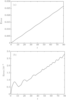
We choose ν = 0.1, τ = 0.01, and h = 0.1. From Fig. 1, one can see that the errors in solution ψ grow nearly linearly while the ones in solution ϕ grow oscillatory. One can also find that figure 1 is very similar to that in Ref. [7]. The local energy and the errors in the global invariants are listed in Table 1. It is clear that the local energy 𝓔 _local is always in the scale of 10^{− 14} throughout computations. Therefore, the local energy is conserved exactly. Since the errors in charge and global energy oscillate near zero in the scale of 10^{− 15}, the two global invariants are also captured.

Fig. 1.

	Figure Option ViewDownloadNew Window
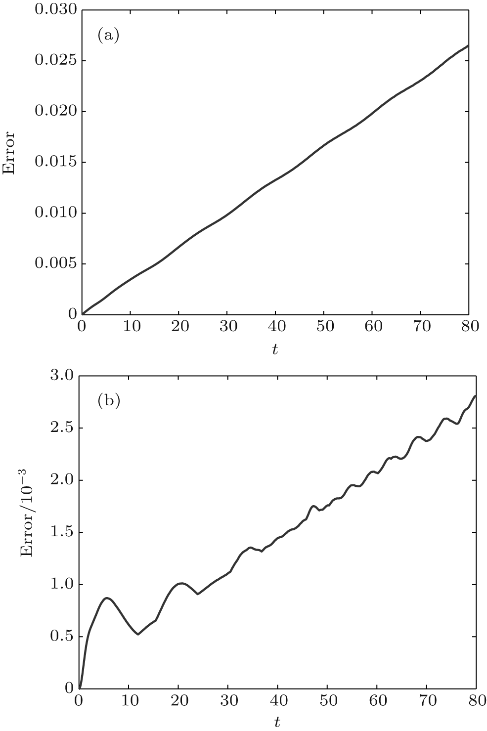	Fig. 1. (a) L∞ (ψ ), (b) L∞ (ϕ ).

Table 1.

Table 1.

Table 1. Local energy and the errors in global invariants for soliton at different time. Time | 𝓔 n – 𝓔 0| /10– 15 | 𝒬 n – 𝒬 0| /10– 16 10 1.42 0.333 4.44 20 2.13 2.88 17.7 40 3.55 3.99 8.88 60 2.13 5.32 62.1 80 2.48 3.10 93.2

Table 1. Local energy and the errors in global invariants for soliton at different time.

Next, we compare the numerical performance of the LEP scheme with that of the existing methods.^{[4, 5, 9]} We implement all methods with ν = 0.3, various temporal and spatial step sizes. Table 2 reports the errors in the solutions, and the changes in charge and global energy at T = 1. From the table, we find that the solutions of LEP are better than those of C-C, M-M, T-C, and T-T schemes, while a little worse than the M-C scheme. The errors in invariants show that our method conserves the charge and the global energy much better than the others.

Table 2.

Table 2.

Table 2. Comparison with some existing methods in numerical error and conserved invariants. τ /h Method L2(ϕ )/10– 4 L2(ψ )/10– 4 | 𝒬 n – 𝒬 0| | 𝓔 n – 𝓔 0| 0.1/0.2 LEP 13.609 31.168 1.7764× 10– 15 5.5511× 10– 16 C-C[4] 14.248 31.348 5.7731× 10– 15 3.4417× 10– 15 M-M[5] 33.417 64.025 4.4409× 10– 15 1.8917× 10– 6 M-C[9] 12.718 30.537 6.9201× 10– 15 1.2436× 10– 6 T-C[9] 13.668 31.750 4.1392× 10– 6 8.4530× 10– 7 T-T[9] 27.508 65.403 8.9399× 10– 16 6.6946× 10– 5 0.05/0.1 LEP 3.6181 8.1743 8.8818× 10– 16 1.1102× 10– 16 C-C[4] 3.7850 8.2222 1.1102× 10– 14 4.5519× 10– 15 M-M[5] 8.8406 16.938 7.5495× 10– 15 1.3297× 10– 7 M-C[9] 3.3875 8.0046 1.2155× 10– 14 7.7985× 10– 8 T-C[9] 3.6365 8.3281 6.7716× 10– 8 8.8421× 10– 8 T-T[9] 7.2219 17.011 4.3669× 10– 7 6.6713× 10– 6

Table 2. Comparison with some existing methods in numerical error and conserved invariants.

Example 2 (solitons collision) In the following simulations, we study head-on collisions of two solitary waves. The initial conditions are chosen as ψ ₀ = ψ (x, 0, v₁, x₁) + ψ (x, 0, v₂, x₂), ϕ ₀ = ϕ (x, 0, v₁, x₁) + ϕ (x, 0, v₂, x₂), and ϕ ₁ = ϕ _t(x, 0, v₁, x₁) + ϕ _t(x, 0, v₂, x₂). We consider the simulation over the region [– 40, 40] × [0, 80] with parametersτ = 0.01 and h = 0.1.

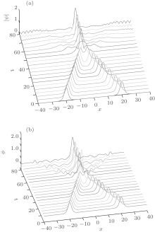
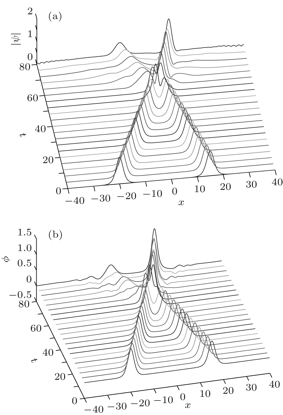
First, we investigate the collision of symmetric solitons, i.e., ν ₁ = 0.4, x₁ = – 20 and ν ₂ = – 0.4, x₂ = 20. Figure 2 displays the evolution of ψ and ϕ . The two solitons collide at about T = 40, and then seem to be trapped. Table 3 displays the local energy, and the errors in charge and global energy against time. The results coincide with the theoretical analysis.

Fig. 2.

	Figure Option ViewDownloadNew Window
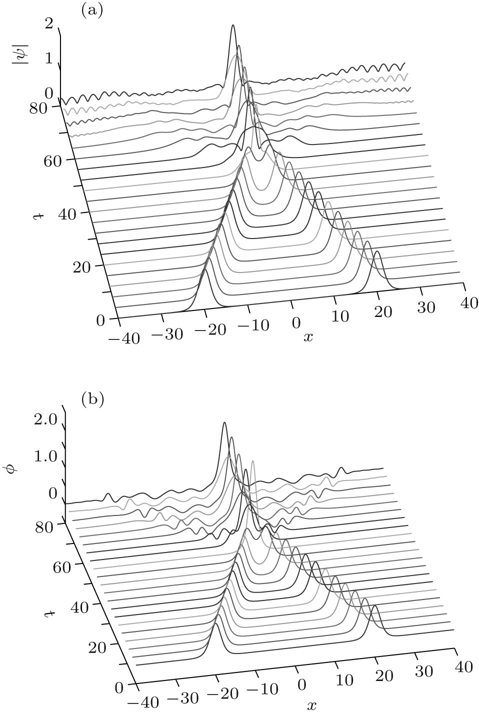	Fig. 2. Symmetric solitons collision: (a) | ψ | , (b) ϕ .

Table 3.

Table 3.

Table 3. Local energy, and the errors in global invariants for symmetric solitons collision at different time. Time | 𝓔 n – 𝓔 0| /10– 15 | 𝒬 n – 𝒬 0| /10– 15 10 4.97 2.55 5.32 20 4.26 16.8 7.10 40 3.19 66.0 17.7 60 4.26 13.0 17.7 80 17.0 19.3 17.7

Table 3. Local energy, and the errors in global invariants for symmetric solitons collision at different time.

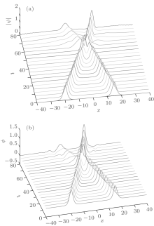
Second, we consider the non-symmetric solitions collision with ν ₁ = 0.4, x₁ = – 20 and ν ₂ = – 0.2, x₂ = 15. The simulation results are illustrated in Fig. 3. It is clear that the soliton with the larger amplitude becomes larger and the one with the smaller amplitude becomes smaller after the collision. The local energy 𝓔 _local, and the errors in charge and global energy are presented in Table 4. The results are all within the roundoff error of the machine. Again the proposed LEP scheme conserves the invariants exactly.

Fig. 3.

	Figure Option ViewDownloadNew Window
	Fig. 3. Non-symmetric solitons collision: (a) | ψ | , (b) ϕ .

Table 4.

Table 4.

Table 4. Local energy, and the errors in global invariants for non-symmetric solitons collision at different time. Time | 𝓔 n – 𝓔 0| /10– 15 | 𝒬 n – 𝒬 0| /10– 16 10 4.26 25.5 62.1 20 3.55 26.6 8.88 40 4.26 15.9 97.7 60 11.3 15.9 133 80 8.52 1.11 142

Table 4. Local energy, and the errors in global invariants for non-symmetric solitons collision at different time.

In this work, we propose a LEP scheme to simulate the KGS equations. The local property is independent of the boundary conditions. Our method preserves the discrete LECL in any time– space region. If the boundary conditions are suitable, the LEP method will be the GEP method. Therefore, the method in the present paper extends the applying scope of the traditional GEP algorithm. Numerical results indicate that the present scheme can provide accurate solutions in long-term computations, and also show excellent performance in conserving the local energy, global energy, and charge invariants. From Eq. (5), we can also derive local momentum and global momentum conservation laws for the KGS equations. As we know, they are also important invariants in physics. Similarly, we could consider local momentum-preserving schemes for the KGS equations.