The human immunodeficiency virus (HIV) infectious disease has been a huge threat to human health with its high rate of global spread. HIV mainly attacks CD4⁺ T cells which are major components of the human immune system. During the HIV infection period there is an increase in the infected CD4⁺ T cell and a decrease in the CD4⁺ T cell count.^[1] Once the CD4⁺ T cell count is lower than 200  mm^{− 3} in an HIV infected person, this patient is classified as having AIDS.^[2] Mathematical models of epidemic dynamics have been developed to improve our understanding of the disease, and much work has been done by researchers.^{[3– 7]} Martin and Charles^[8] developed population dynamics models by exploring the relation between antiviral immune responses, virus load, and virus diversity. Patrick and Alan^[9] analyzed a set of models that include intracellular delays, combination antiretroviral therapy, and the dynamics of both infected and uninfected T cells.

The basic mathematical model^{[1, 2, 10, 11]} of HIV infection includes three state variables: uninfected CD4⁺ T-cells T, infected cells I, and free virus particles V as follows:

Here the parameter S is the total rate of production of healthy cells per unit time; b, a, and c are the per capita death rates of healthy cells, infected cells, and infective virus particles respectively. The infection is represented by a mass action term KTV; α is the viral production rate of an infected cell. Much work regarding the pathogenesis of HIV in-host has been done using this basic model, and many extended models have been developed to understand and analyze the dynamics of an HIV infection. Global dynamics of system (1) has been analyzed by the basic reproduction number R₀ = Kα S/abc.^[12] D’ Onofrio^[13] assumed that the incidence functions should be (1 − γ )β TV and (1 − η )NaI under the influence of highly active antiviral therapy (HAART), and studied the global asymptotic stability of the disease-free equilibrium of the HIV infection model, where β is the transmission coefficient between uninfected cells and infective virus particles, 1 − γ (0 < γ < 1) is the reverse transcriptase inhibitor (RTI) drug effect; and 1 − η (0 < η < 1) is the protease inhibitor (PI) drug effect; N is the average number of infective virus particles produced by an infected cell.

In infectious disease modelling, the model’ s parameters have become a crucial factor to ensure that the models have some realistic significance and may give some reasonable description.^[14] In the previous models, the infection rate K and the viral production rate α are considered to be constant coefficients. However, they are time-varying due to the effect of RTI and PI drugs. Drugs are most commonly prescribed to be taken on a fixed dose, fixed time interval basis. The drug efficacy function is usually characterized by a rapid rise to a peak value after drug intake, followed by a slower decay.^[15] Browne and Pilyugin^[16] assumed that the drug efficacy functions are bang– bang type, i.e., either it is active at a fixed efficiency level, or it is inactive, and studied the stability of the infection free steady state by the basic reproduction number. Liu and Stechlinski^[17] analyzed infectious disease models with time-varying parameters and obtained some sufficient conditions to ensure the stability of the disease-free equilibrium. Wang et al.^[18] assumed that incidence functions are time-varying functions and switching functional forms in time, analyzed the extinction of the disease. Motivated by the discussion, assume that both the infection rate and viral production rate are time-varying function and switching forms in time. The model is called a switched HIV model. For the switched system, one main feature is that the included switching law may induce stability of the switched system composed of two unstable subsystems.^{[21– 23]} We will use some of the switched systems techniques^[41] to establish the threshold conditions of the disease eradiation and persistence.

In recent years, researchers have added many factors (such as delay, treatment) to describe the immunological response to infection with HIV and make predictions about their dynamics.^{[19, 20, 24, 25]} Stochasticity, as one of the most important factors in the structure and function of biological systems, has been introduced by a fluctuating environment or other ways. Stochastic HIV models have been concerned with the study of Gaussian noise.^{[26– 29]} Experimental evidence, particularly in biological virus systems, indicates that most of the noises are not only Gaussian white noise, but also non-Gaussian noise, or bounded noise, or combined Gaussian white noise.^{[30– 34]} Jiang et al.^[35] investigated dynamical behavior of a tumor-growth model with coupling non-Gaussian and Gaussian noise terms. Sebastiano et al.^[36] modeled extrinsic fluctuations in biomolecular networks by means of bounded noise. For different cells, there appear different cell growth and decay processes. Thus, we will study the dynamics of the switched HIV model subjected to combined bounded noise and Gaussian white noise, which are introduced by replacing the death rate parameters of healthy cells and infected cells.

The paper is organized as follows. In Section  2, we first outline the extended HIV dynamics model. New threshold conditions are established to examine the disease extinction or persistence from the stochastic switched dynamical view point. In Section  3, numerical simulations are given to illustrate our results. Some conclusions are given in Section  4.

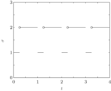
Consider a family of m different infection rates with the general form K_i with i = 1, 2, ..., m. Assume that the infection rate is modeled as a switching parameter and is governed by a switching rule σ , where σ ∈ { 1, 2, ..., m} is a piecewise constant function of time, continuous from the left. That is, σ = i indicates that the i-th subsystem is activated. Corresponding to the switching rule σ (t), the i_k-th subsystem is activated when t ∈ (t_{k− 1}, t_k]. Denote the set of all such switching rules by 𝒥 . A switching rule example for the switched infection rate is as follows: suppose that K is equal to K₁ in the 1st subsystem and K is equal to K₂ in the 2nd subsystem. This gives the following switching rule, as illustrated in Fig.  1:

Fig.  1.

	Figure Option ViewDownloadNew Window
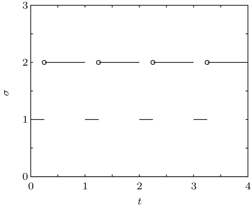	Fig.  1. The periodic switching rule (2).

Furthermore, assume that the reproductive rate of the infected cells is a switching parameter α _i. The switching parameters are also assumed to be governed by the above switching rule σ . Under the above assumptions, this leads to a new switched HIV model,

with the initial conditions T(0) = T₀, I(0) = I₀, and V(0) = V₀. System (3) has a disease-free equilibrium E₀ = (S/b, 0, 0), and endemic solution in the i-th subsystem, where satisfy the following equations:

The basic reproduction number R₀ becomes an important tool to study the dynamics of epidemic models, and can be defined as the average number of secondary cases produced by a single infective population introduced into an entirely susceptible population. For the switched HIV epidemic model (3), the basic reproduction number R₀ can be the spectral radius of a next generation integral operator, R₀ = ρ (L), where the next infection operator L is given by^{[38, 39]}

where Φ is a continuous function and P(t, x) is the rate of new infections produced by the infected individuals who were introduced at time t – x.

According to the fact that the dynamics of the viral particles are much faster than the dynamics of cells, we make a quasi-steady state assumption for the third equation of system (3) (see Refs.  [1] and [37]), i.e.,

Then system (3) can be rewritten as

This system has a solution Q = (S/b, 0). Introduce randomness into the above model by replacing the parameters b and a by b → b + ξ (t) and a → a + ϕ W(t). Hence, we obtain the following system:

where ξ (t) is a bounded noise of the form ξ = A sin(Ω t + ϕ W(t) + U). Here A, Ω , and ϕ are positive constants; A and Ω are the amplitude and center frequency of bounded noise; ϕ is an intensity parameter of random frequency; W(t) is the standard Wiener process; and U is a random phase uniformly distributed in [0, 2π ].

Definition 1^[40] The population X(t) is said to go to extinction if .

Definition 2^[40] The population X(t) is said to be weakly persistent in the mean if .

Lemma 1 Consider system (6) for any initial value , there is a unique solution (T(t), I(t)) on t ≥ t₀ and the solution will remain in with probability 1, where .

Proof The proof is similar to that in Refs.  [28] and [42], and omitted here.

Note that drugs are commonly prescribed to be taken on a fixed dose, fixed time interval. The effect of the drug varies during the treatment cycle. Consider a periodic switching rule, which is constructed as that of Ref.  [41]. Assume that the switching rule σ satisfies t_k− t_{k− 1} = ω _k with ω _{k+ m} = ω _k. Assume that K_{k+ m}(t) = K_k(t) and K_k(t) = K_k(t + ω ), where ω = ω ₁ + ω ₂ + · · · + ω _m is a period of the switching rule. Denote the set of all switching rules satisfying these properties by 𝒥 _periodic ⊂ 𝒥 .

Theorem 1 Assume that the switching rule σ is periodic, and b > A. If R̄ ₀ < 1 where

then the disease goes to extinction with probability 1.

Proof Under the condition of R̄ ₀ < 1 it follows that there exists ε > 0, such that

From Eq.  (6) we have

It follows that T(t) ≤ S/(b− A). Furthermore, for t ∈ (t_{k− 1}, t_k], let y(t) = log I(t). Applying Itô formula, we obtain

where f_σ = α _σ K_σ /c. Noting that y(t) is Brown motion, it follows that

namely,

Take the expectation of I(t) for Eq.  (12), then

Since I(t₀) is independent of W(t)− W(t₀), then for t ∈ (t₀, t₁],

Noting that , it follows that

In general, for t ∈ (t_{k− 1}, t_k] follows that

When t = t₀ + ω , it follows that

where

Note that the switching rule σ is periodic, then for some integer h = 1, 2, ..., E(I(t₀ + hω )) ≤ η E(I(t₀ + (h − 1)ω )) ≤ · · · ≤ η ^hME(I(t₀)) = η ^hMI(t₀).The sequence {E(I(t₀ + hω ))} → 0, h → ∞ . Hence, it can be concluded that the disease goes to extinction with probability 1.

Corollary 1 Assume that the switching rule σ ∈ 𝒥 and b > A. If R̄ ₀ < 1 where

for some l ≥ t₀, then the disease goes to extinction with probability 1.

Remark 1 We know if the basic reproduction number is larger than the one in the subsystem, then this subsystem is unstable. However, if the amplitude A is smaller and the condition R̄ ₀ < 1 is satisfied, then all solutions of system (6) converge to the disease-free equilibrium Q, which implies that system (6) is stable.

Remark 2 In the special case that parameters of system (6) are constant and A = ϕ = 0, then the basic reproduction number R̄ ₀ of system  (6) is reduced to R₀.^{[1, 2, 10, 11]}

Remark 3 We see that, for A = ϕ = 0 (i.e., there is no noise for the death rates),

guarantees the disappearance of the disease, which agrees well with the classical results.

Remark 4 Compared with the model (1.2) proposed in Ref.  [5], the results in this paper are more explicit. When K_σ = K(t) and α _σ = Nδ , we can derive that

Theorem 2 Assume that the switching rule σ is periodic, and R̂ ₀ > 1, where

then the disease weakly persists with a probability of 1.

Proof Assume that for a given . Under this assumption, for t ∈ (t_{k− 1}, t_k],

where

with f_σ = α _σ K_σ /c.Consider the following equation:

whose solution converges to S/(b + f* ɛ + A). For the choice of ε above, there exists a time t* > t₀, such that T(t) ≥ S/(b + f* ɛ + A) − ɛ . Furthermore, for t* < t_{k− 1} < t ≤ t_k, let Y(t) = logI(t). Applying Itô formula, it follows that

Since Y(t) is Brown motion, it follows that

i.e.,

Taking the expectation of I(t) for Eq.  (24), it follows that

Note that I(t₀) is independent of W(t) − W(t₀), then for t ∈ (t₀, t₁],

Noting that

we have

In general, for t* + (k − 1)ω < t ≤ t* + kω , it follows that

where . Choose

Note that , which is a contradiction. Therefore, the disease weakly persists.

Corollary 2 Assume that the switching rule σ ∈ 𝒥 , and R̂ ₀ > 1, where

for l ≥ t₀, then the disease weakly persists with probability 1.

Remark 5 The condition R̂ ₀ > 1 in Theorem 2 is a much less restrictive condition as the basic reproduction number of the disease may be less than one during some intervals.

Remark 6 From Theorems 1 and 2, we can see that the disease will die out when R̂ ₀ > 1, and the disease will persist when R̂ ₀ > 1. Furthermore, it is worth pointing out that R̂ ₀ > R̄ ₀

In order to illustrate the effectiveness of the proposed results above, the dynamics of the HIV models with two types of noise and switching functions is presented. For these simulations, most of these values have been taken from published literature. b, a, c have been taken from Ref.  [1], S from Ref.  [43]. We choose appropriate values for K_i and α _i, as the same as those in Ref.  [12]. More specifically, let the parameter values be S = 10⁴  day^{− 1}· dm^{− 3}, b = 0.5  day^{− 1}, a = 1.9  day^{− 1}, c = 3  day^{− 1}. Take switching parameters (I): α ₁ = 0.56, α ₂ = 0.46, K₁ = 10^{− 4}  day^{− 1}· dm^{− 3}, and K₂ = 10^{− 3}  day^{− 1}· dm^{− 3}. Assume that t₀ = 0, and the switching law is periodic and satisfies

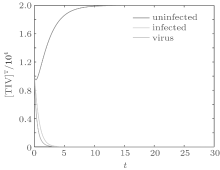
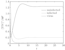
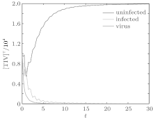
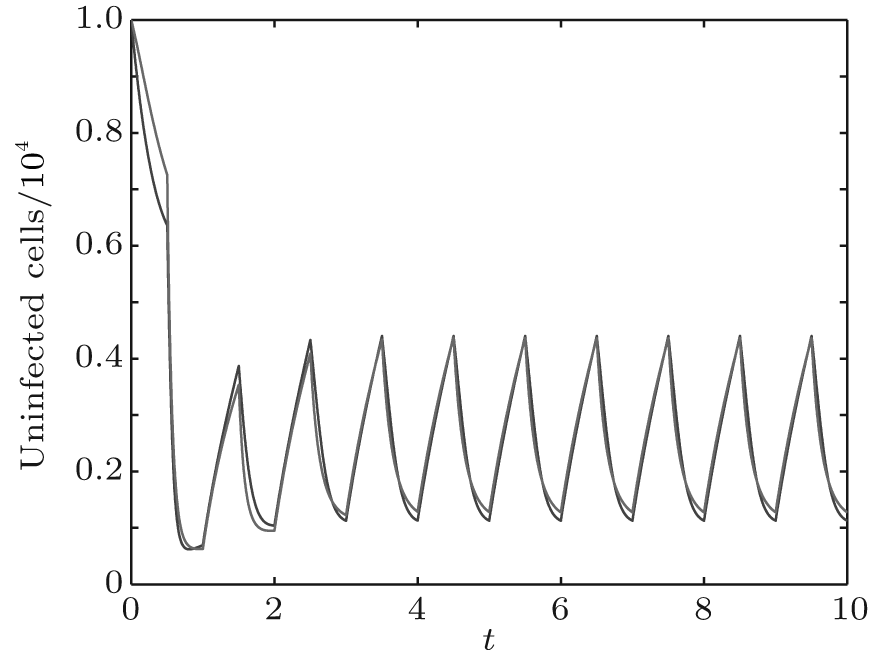
We first performed simulation for systems (1) and (3) to show the effect of the switching functions on an HIV infection. We choose the switching parameters (I) for system (3), and choose two sets of parameters (II): α = α ₁, K = K₁; (III): α = α ₂, K = K₂ for system  (1), respectively. When taking parameter (II), numerical calculations show that the solutions of system  (1) converge to the disease-free equilibrium (2× 10⁴, 0, 0), which implies that the disease dies out (see Fig.  2). When taking parameter (III), figure  3 shows that the solutions of system (1) do not converge to the disease-free equilibrium (2× 10⁴, 0, 0), which implies that the disease is persistent. However, taking the switching parameter (I), it is clearly seen from Fig.  4 that the switched HIV model (3) approaches the disease-free equilibrium (2× 10⁴, 0, 0), which implies that system  (3) is stable, regardless of whether the subsystem is unstable or stable. Besides, we performed simulation for systems (3) and (5) in order to demonstrate the reasonability of the quasi steady-state assumption on the free virus. Computer simulations agree well with mathematical analysis results (see Figs.  5 and 6).

Fig.  2.

	Figure Option ViewDownloadNew Window
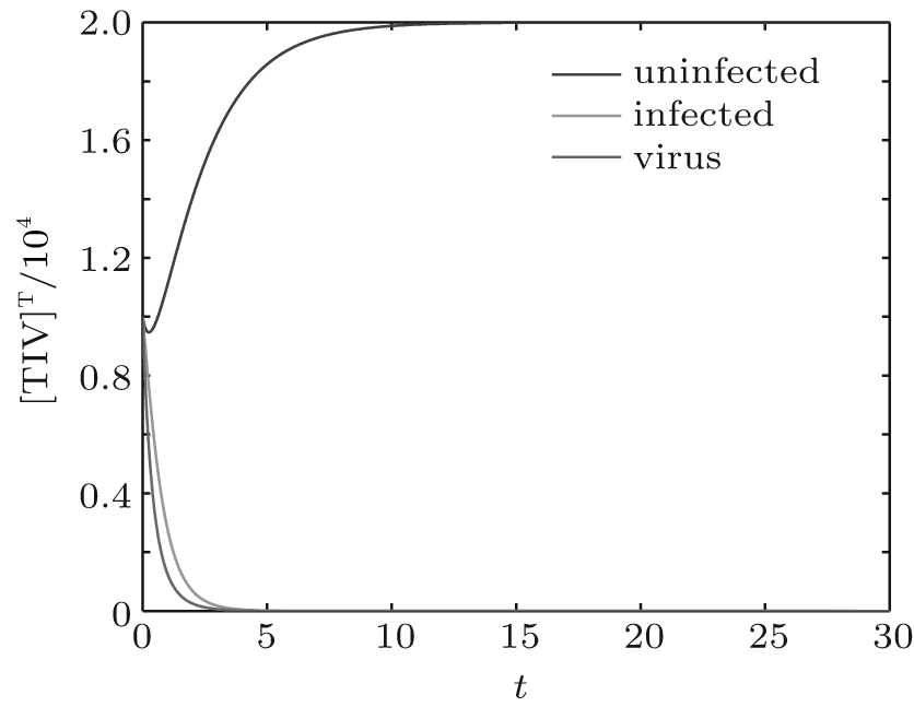	Fig.  2. Solutions of system (1) with parameter (II).

Fig.  3.

	Figure Option ViewDownloadNew Window
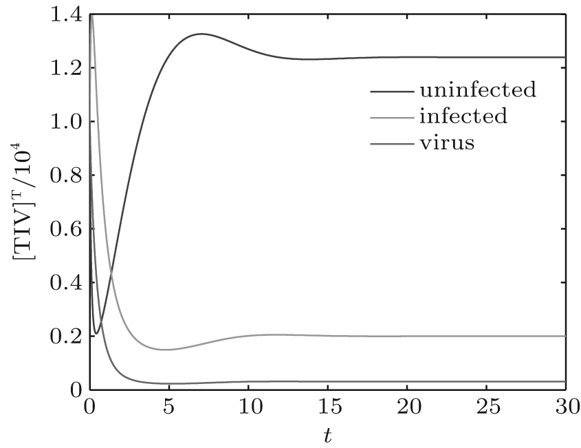	Fig.  3. Solutions of system (1) with parameter (III).

Fig.  4.

	Figure Option ViewDownloadNew Window
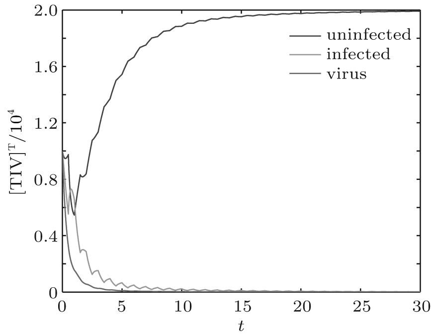	Fig.  4. Solutions of system (3) with parameter (I).

Fig.  5.

	Figure Option ViewDownloadNew Window
	Fig.  5. Solutions of uninfected cells for systems (3) and (5).

Fig.  6.

	Figure Option ViewDownloadNew Window
	Fig.  6. Solutions of infected cells for system (3) and system (5).

Let the parameters be A = 0.001, Ω = 0.2, and ϕ = 0.5, the switching parameters be α ₁ = 0.36, α ₂ = 0.46, K₁ = 10^{− 4}  day^{− 1}· dm^{− 3}, and K₂ = 10^{− 3}  day^{− 1}· dm^{− 3}, and keep all other parameters unchanged. This gives the basic reproduction number of the two subsystems: R₁ = 0.1266 < 1, R₂ = 1.463 > 1. Based on Theorem  1, we can derive that. Then, we can draw the conclusion that the disease dies out (see Fig.  7). On the other hand, let the parameter values be A = 0.02, Ω = 0.2, and ϕ = 0.5, choose the switching parameters α ₁ = 0.26, α ₂ = 0.46, K₁ = 10^{− 3}  day^{− 1}· dm^{− 3}, and K₂ = 10^{− 2}  day^{− 1}· dm^{− 3}, and other parameters are unchanged. We can derive that the basic reproduction numbers of each subsystem are R₁ = 0.8772 < 1 and R₂ = 15.5196 > 1, then R̂ ₀ = 8.1984 > 1. According to Theorem  2, the disease persists. Figure  8 shows that the simulation agrees very well with the theoretical analysis result.

Fig.  7.

	Figure Option ViewDownloadNew Window
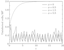
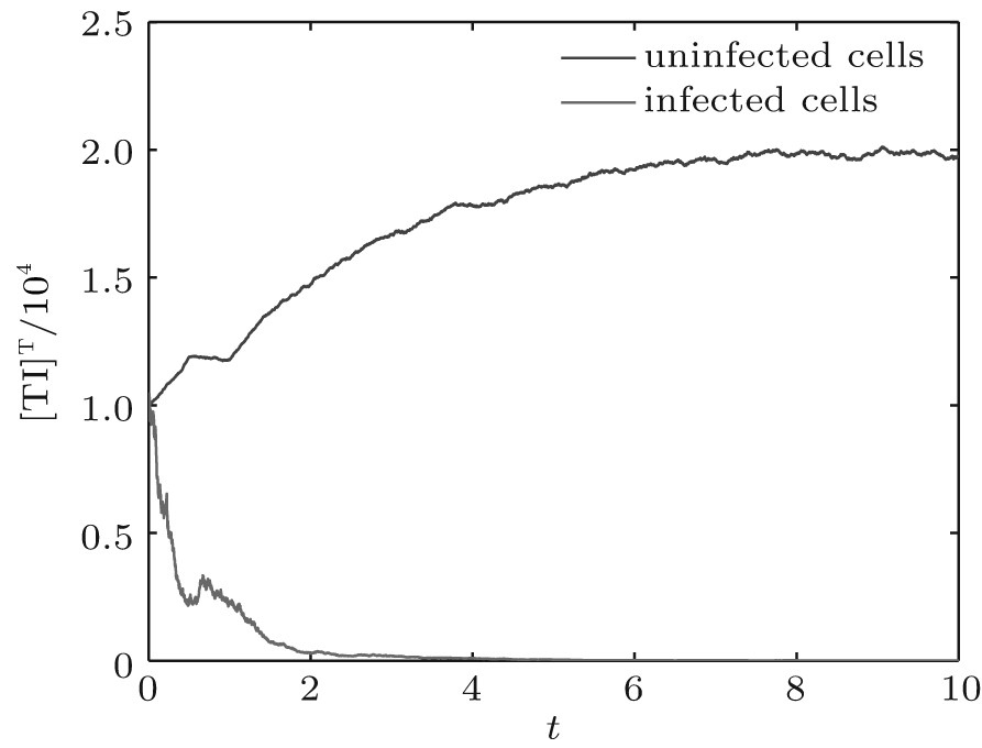	Fig.  7. Solutions of system (6).

Fig.  8.

	Figure Option ViewDownloadNew Window
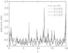
	Fig.  8. Solutions of system (6).

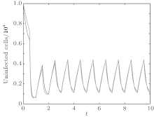
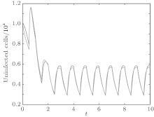
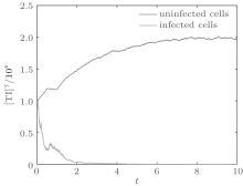
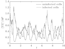
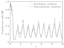
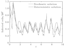
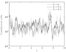
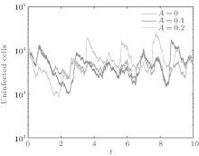
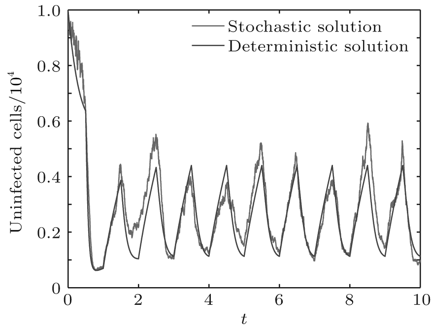
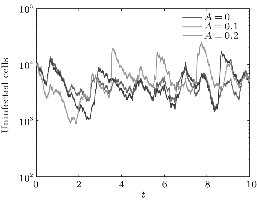
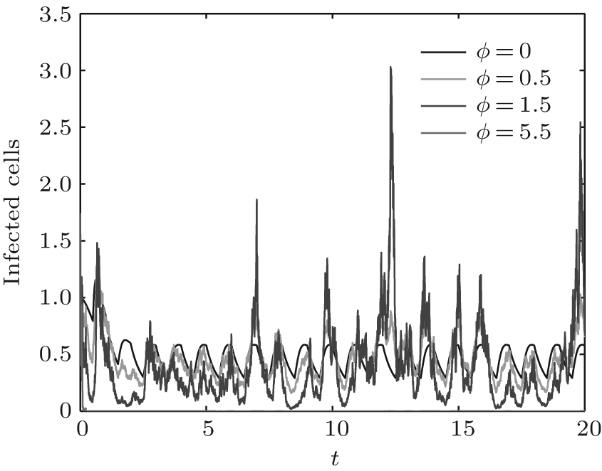
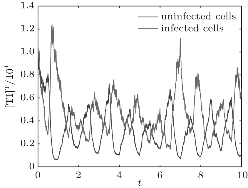
In order to illustrate some of the effects of bounded noise and Gaussian white noise on the switched HIV model, we numerically solve the model (6) and its corresponding deterministic model (5). Let the parameter values be A = 0.02, Ω = 0.2, and ϕ = 0.5, choose the switching parameters α ₁ = 0.56, α ₂ = 0.46, K₁ = 10^{− 3}  day^{− 1}· dm^{− 3}, and K₂ = 10^{− 2}  day^{− 1}· dm^{− 3}, and other parameters are unchanged. As can be clearly seen from Figs.  9 and 10 that the stochastic solutions of Eq.  (6) always fluctuate around the solutions of system (5), and the stochastic perturbation do not change the persistence of the disease. In Figs.  11 and 12, the fluctuation reduces as the amplitude of bounded noise A decreases if ϕ is fixed and other parameters are unchangeable. When A is fixed and we only change ϕ , figure  13 shows that the increase in stochastic noise intensity ϕ can lead to higher peaks of the uninfected cells and then stay close to the equilibrium state. Infected cells decrease as the intensity of noise intensity ϕ increases (see Fig.  14), which implies that strong noise intensity may cause the disease to die out.

Fig.  9.

	Figure Option ViewDownloadNew Window
	Fig.  9. Solutions of uninfected cells for systems (5) and (6).

Fig.  10.

	Figure Option ViewDownloadNew Window
	Fig.  10. Solutions of infected cells for system (5) and system (6).

Fig.  11.

	Figure Option ViewDownloadNew Window
	Fig.  11. Solutions of uninfected cells for system (6).

Fig.  12.

	Figure Option ViewDownloadNew Window
	Fig.  12. Solutions of infected cells for system (6).

Fig.  13.

	Figure Option ViewDownloadNew Window
	Fig.  13. Solutions of uninfected cells for system (6).

Fig.  14.

	Figure Option ViewDownloadNew Window
	Fig.  14. Solutions of infected cells for system (6).

In this paper, new HIV models with switching functions and combined bounded noise and Gaussian white noise are presented and studied. The model’ s parameters are first assumed to be time-varying functions and switching functional forms in time. Stochasticity is considered by parameter perturbations. The basic HIV model can be extended to the stochastic switched HIV model. Furthermore, new sufficient conditions are established to measure the extinction or persistence of the disease on the basis of the Razumikhin-type approach. The results show that the disease will die out when the new basic reproduction number R̄ ₀ is less than 1 and the amplitude of bounded noise is smaller; the disease is persistent in the mean when the new basic reproduction number R̂ ₀ is greater than 1. Different stochastic noises have different effects on the dynamics of the epidemic model. The disease will disappear and all CD4⁺ T cells are uninfected cells if the intensity ϕ of the Gaussian noise becomes large enough.