In heat conduction problems, when the heat flux and/or temperature histories at the surface of a solid body are known as functions of time, then we find the temperature distribution. This is termed as a direct problem. However, in many heat transfer situations, the surface heat flux and temperature histories must be determined from temperature measurements at one or more interior locations. This is an inverse problem. Inverse heat conduction problems (IHCPs) play a very important role in many branches of science and technology. The problem consists in determining the temperature and heat flux. The IHCP is much more difficult to solve than the direct heat conduction problem in which the initial and boundary conditions are given and the temperatures are to be determined. This IHCP equation is analyzed in the literature.^{[1– 14]} Hetmaniok et al.^[1] applied the homotopy perturbation method for the solution of inverse heat conduction problem. Moreover, Slota^[2] implemented homotopy perturbation method for the solution of one phase. A hybrid inverse scheme was applied by Chen and Wu^[3] for estimation of surface conditions for nonlinear IHCPs. Cialkowski et al.^[4] used Trefftz non-continuous method for the solution of a stationary inverse heat conduction problem. Kalman filter-enhanced Bayesian back propagation was successfully applied by Deng and Hwang^[5] to obtain the solution of IHCPs. Frackowiak et al.^[6] developed the fitting algorithm for the solution of inverse problems of heat conduction. Different finite element methods were used by Grvsa and Lesniewska^[7] for the solution of IHCPs. Grzymkowski and Slota^[8] solved one-phase inverse Stefan problems by the Adomian decomposition method. The Laplace transform was used by Monde et al.^[9] to obtain the solution of two-dimensional inverse heat conduction problems. Wroblewska et al.^[10] implemented the modified method of elementary balances to obtain the numerical solution of a direct and inverse heat transfer problem. Woodfielda et al.^[11] presented the solution of two-dimensional inverse heat conduction problem. An analytical solution based on Greens function has been obtained by Fernandes et al.^[12] to reduce computational time in inverse heat conduction problems. The lattice Boltzmann method was used by Kameli and Kowsary^[13] to obtain the solution of inverse heat conduction problem. Johansson et al.^[14] proposed a new method to obtain the solutions for the radially symmetric inverse heat conduction problem.

In all of the above cited papers, we may observe that the authors have considered the parameters and the initial/boundary conditions as crisp or defined exactly. In addition, many other authors^{[15– 32]} have also investigated some application problems with crisp variables and parameters. However, in actual practice, rather than the particular value, only uncertain or vague estimates about the variables and parameters may be known. This is because these are found in general by some observations, experiments, or experiences. Hence, to handle these uncertainties and vagueness, one may use interval or fuzzy parameters and variables in the governing differential equations. In this context, some papers related to fuzzy differential equations are given in Refs.  [33]– [37]. The concept of fuzzy derivative was first introduced by Chang and Zadeh.^[33] It was followed by Dubois and Prade.^[34] The fuzzy differential equations and fuzzy initial value problems were studied by Kaleva^[35] and Seikkala.^[36] The analytical method is developed by Bede^[37] using the Hukuhara derivative to obtain the solution of fuzzy differential equations. Various numerical methods for solving fuzzy differential equations are also introduced in Refs.  [38]– [46]. Ma et al.^[38] developed a scheme based on the classical Euler method to solve the fuzzy ordinary differential equations. A two-dimensional differential transform method to solve fuzzy partial differential equations (FPDEs) has been studied by Mikaeilvand and Khakrangin.^[39] An algorithm based on α - cut of a fuzzy set has been developed by Akin et al.^[40] for the solution of second-order fuzzy initial value problems. Variation of constant formula is handled by Khastan et al.^[41] to solve first-order fuzzy differential equations. The concept of generalized H-differentiability is studied by Chalco-Cano and Roman Flores^[42] to solve fuzzy differential equations. Behera and Chakraverty^[43] obtained the uncertain impulse response of an imprecisely defined half-order mechanical system. Also, the fuzzy hyperbolic reaction-diffusion equation was solved by Tapaswini and Chakraverty^[44] to analyze the uncertain forest fire. A new double parametric form of fuzzy number has been developed by Tapaswini and Chakraverty, ^[45] and then they applied the Adomian decomposition method to obtain the solution of uncertain vibration equation for very large membranes.

Recently, the variational iteration method (VIM) is found to be a powerful tool for the analysis of linear and non-linear physical problems. The VIM was first developed by He^{[46, 47]} and was successfully applied to solve various linear and non-linear differential equations of scientific and engineering problems. Convergence of the VIM is proved in Ref.  [48]. Very recently, VIM has been applied to a wide class of other physical problems.^{[49– 55]}

In the present analysis, VIM is applied for the numerical solution of the uncertain inverse heat conduction problem. Uncertainty in the initial condition is defined in term of fuzzy numbers. Our literature review reveals that fuzzy differential equations are always converted to two crisp differential equations in general to obtain the solution bounds. However, in the proposed methodology the fuzzy differential equation has been converted to a single crisp differential equation using double parametric form of fuzzy numbers^[45] and then the corresponding crisp differential equation is solved to obtain the final fuzzy solution by substituting the parametric values.

This paper is organized as follows. In Section 2, some basic preliminaries related to the present investigation are given. In Section 3, the basic idea of the VIM is discussed. The VIM is applied with the proposed technique in Section 4 to solve uncertain inverse heat conduction problems. In Section 5, fuzzy and interval solutions for different types of initial conditions are given.

In this section, we present some notations, definitions, and preliminaries, which are used further in this paper.^{[56– 60]}

Definition 1. Fuzzy number A fuzzy number Ũ is a convex normalized fuzzy set Ũ of the real line R such that

where μ _Ũ is called the membership function of the fuzzy set and it is piecewise continuous.

Definition 2. Triangle fuzzy number A fuzzy number Ũ is said to be triangular if

(i) there exists exactly one x₀ ∈ R with μ _Ũ (x₀) = 1 (x₀ is called the mean value of Ũ ), where μ _Ũ is called the membership function of the fuzzy set; (ii) μ _Ũ (x) is piecewise continuous.

Let us consider an arbitrary triangular fuzzy number Ũ = (a, b, c). The membership function μ _Ũ of Ũ will be defined as follows:

Definition 3. Singular parametric form of fuzzy number The triangular fuzzy number Ũ = (a, b, c) in single parametric form can be represented as

where r ∈ [0, 1]. It may be noted that the lower and upper bounds of the fuzzy numbers satisfy the following requirements:

(i) u(r) is a bounded left continuous non-decreasing function over [0, 1],

(ii) ū (r) is a bounded right continuous non-increasing function over [0, 1], and

(iii) u(r) ≤ ū (r), 0 ≤ r ≤ 1.

Definition 4. Fuzzy arithmetric For any two arbitrary fuzzy numbers and ỹ = [y(r), ȳ (r)] and scalar k, the fuzzy arithmetic is defined as follows:

(i) if and only if and ,

(ii),

(iii), where ,

(iv)

Definition 5. Double parametric form of fuzzy number Using the parametric form as discussed in Definition 3 we have Ũ = [u(r), ū (r)]. Now one may write this in double parametric form as Ũ (r, β ) = β (ū (r) − u(r)) + u(r), where r and β ∈ [0, 1].

We consider the uncertain heat conduction equation in the domain D as

where a is the thermal diffusivity, ũ is the uncertain temperature, and t and x refer to time and spatial location, respectively.

Let the domain be defined in R² as D = {(x, t) : x ∈ [0, b], t ∈ [0, t* )} and t* denote the end of the process. On the boundary of the domain, three components are distributed as^[1]

where the initial and boundary conditions are given. On the boundary Γ ₀, the uncertain initial condition is defined as

On the boundary Γ ₁ the uncertain Dirichlet boundary condition is assumed as

In the uncertain inverse problem, the temperature distribution ũ (x, t) in region D along with uncertain temperature and uncertain heat flux ) on boundary Γ ₂ are to be determined. On Γ ₂ we define the Dirichlet and the Neumann boundary condition as

To illustrate the basic idea of the technique, we consider the following general nonlinear system:

where L is a linear operator, N is a nonlinear operator, and g(t) is a given continuous function.

The basic character of the method is to construct a correction functional for Eq.  (6) as follows:

where λ is a general Lagrangian multiplier which can be identified via variational theory, u_n is the n-th approximate solution, and û _n denotes a restricted variation, i.e., δ û _n = 0. The initial approximation u₀ can be freely chosen if it satisfies the initial and boundary conditions of the problem. However, the success of the method depends on the proper selection of the initial approximation u₀ . We approximate the solution as

First we convert the uncertain heat conduction equation to an interval based uncertain heat conduction equation using single parametric form of fuzzy numbers. Then, the interval based differential equation is reduced to crisp differential equation by using double parametric form^[45] of fuzzy numbers. Next, we apply VIM to obtain the solution in double parametric form.

As per the single parametric form, we may write the above fuzzy heat conduction equation as

which subjects to the fuzzy initial condition

Using the double parametric form (as discussed in Definition 5), equation  (8) can be expressed as

subjects to the fuzzy initial condition

where r, β ∈ [0, 1].

Let us now denote

Substituting these into Eq.  (9), we obtain

with the initial condition

Solving Eq.  (10), one may obtain the uncertain temperature as ũ (x, t; r, β ). To obtain the lower and upper bounds of the solution in single parametric form, one may substitute β = 0 and 1, respectively, and thus the solution bounds may be represented as

First we have applied the VIM to solve Eq.  (10). According to VIM, we may construct a correction functional as follows:

By making the above correction functional (i.e., Eq.  (13)) stationary, and noticing that we obtain

Thus, we obtain the Euler– Lagrange equation as

with a natural boundary

Hence, the Lagrange multiplier can be easily identified as follows:

By substituting the identified Lagrange multiplier into Eq.  (13), the following variational iteration formula can be obtained as:

Knowing the uncertain temperature distribution ũ (x, t; r, β ) or its approximation ũ _n(x, t; r, β ), one may easily obtain the missing fuzzy boundary conditions as

In this section we have illustrated the solution procedure by solving some example problems.

Example 1 In this example we consider b = 2, a = 1, and k = 1. The double parametric form of triangular fuzzy initial condition is assumed as

We start with an initial approximation ũ ₀ = ũ (x, 0; r, β ) given by Eq.  (17) and by the variational iterational formula (16), and have

for j ≥ 4.

Therefore, the exact uncertain temperature distribution in the whole region under consideration can be written as

Knowing the uncertain temperature distribution in the whole area, one can easily determine the functions describing the fuzzy boundary conditions as

To obtain the solution bound, i.e., uncertain temperature distribution in single parametric form, we may put β = 0, 1 for lower and upper bounds of the solution, respectively. Hence, we obtain

We have the function describing the boundary condition in term of bounds as

and

One may note that in the special case, when r = 1, the results (crisp) obtained by the proposed method are exactly the same as that of the solution obtained by Hetmaniok et al.^[1] in crisp case.

Example 2 Next, let us take b = 1.2, , k = 2, and the triangular double parametric form of the fuzzy initial condition as

Again, by applying the procedure discussed previously, we obtain the uncertain temperature distribution as

and so on. In the similar manner, higher components of the iteration formula  (16) can be obtained. Finally, the approximate solution may be written as

One can now try to make a higher number of iterations, which result in the convergence of ũ _n = (x, t; r, β ) to the exact solution

The corresponding boundary conditions are found to be

By putting β = 0, 1 into ũ (x, t; r, β ), we may obtain the approximate solution of lower and upper bounds, respectively, as

and

Similarly, we obtain the function describing the boundary condition in terms of bounds as

It is interesting to note again that the exact solution obtained by the proposed method for r = 1 agrees completely with that of the exact solution (crisp result) given by Hetmaniok et al.^[1] in the crisp case.

Numerical results for uncertain inverse heat conduction problems with different fuzzy initial conditions are computed. Obtained results of the present analysis are compared with the existing solution of Hetmaniok et al.^[1] in special case (r = 1). The computed results are shown in figures and tables.

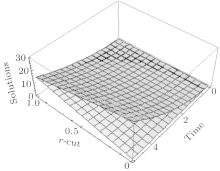
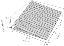
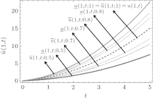
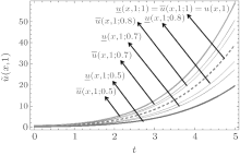
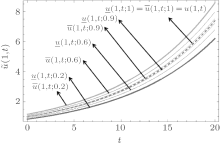
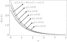
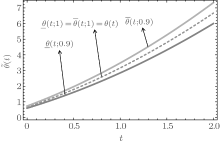
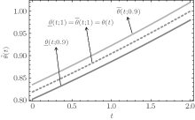
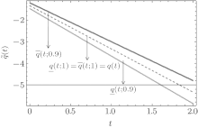
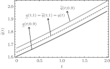
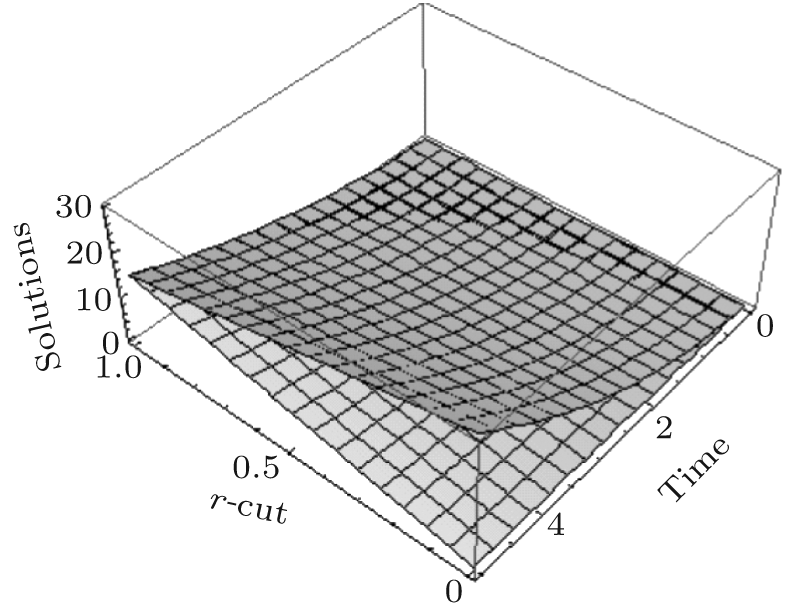
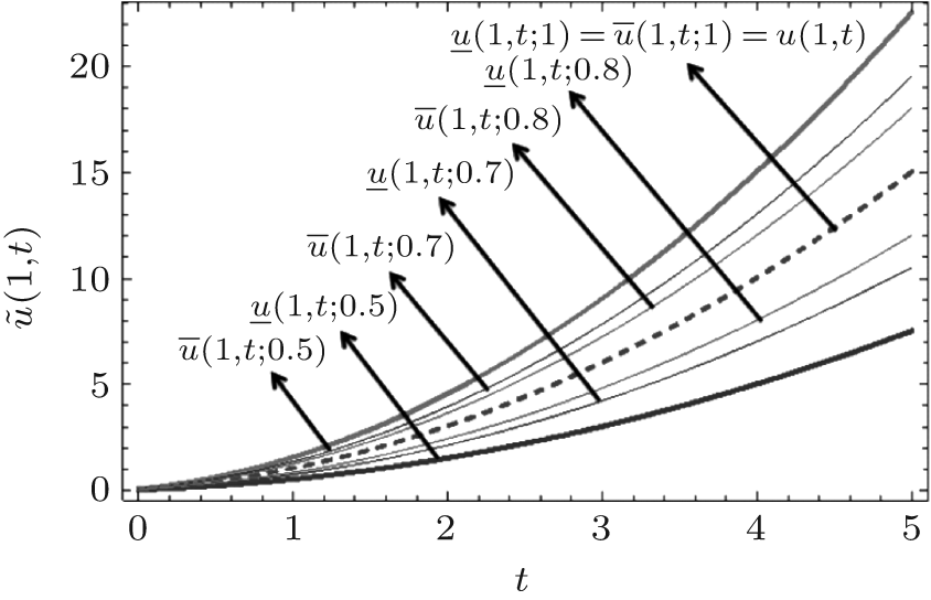
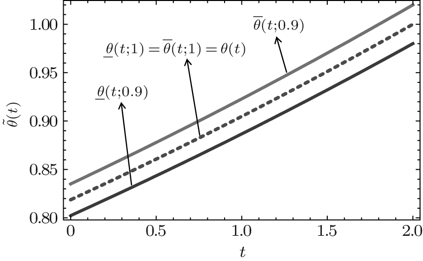
Fuzzy solutions for both Examples  1 and 2 are depicted in Figs.  1 and 2 by varying t from 0 to 5 and keeping x = 1 as constant, respectively, with α = 0.4, 0.6. Interval solution plots for both the examples have been given in Figs.  3– 6. It is also interesting to note from Figs.  3 and 4 that the left and right bounds of the uncertain temperature, i.e., ũ (x, t), (with particular values of x = 1 and t = 1) gradually increase with the increase in t and x, respectively. Solution bounds (viz. interval solution) for uncertain temperature and heat flux on boundary Γ ₂ for r = 0.9 are shown in Figs.  7 and 8 and Figs.  9 and 10, respectively, for both of the examples.

Fig.  1.

	Figure Option ViewDownloadNew Window
	Fig.  1. Fuzzy solution of Example 1 for x = 1.

Fig.  2.

	Figure Option ViewDownloadNew Window
	Fig.  2. Fuzzy solution of Example 2 for x = 1.

Fig.  3.

	Figure Option ViewDownloadNew Window
	Fig.  3. Interval solutions for Example 1.

Fig.  4.

	Figure Option ViewDownloadNew Window
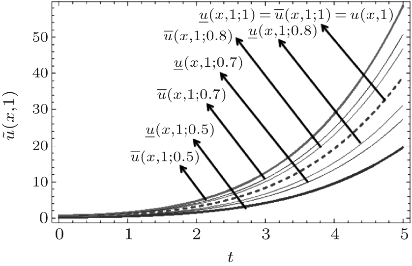	Fig.  4. Interval solutions for Example 1.

Fig.  5.

	Figure Option ViewDownloadNew Window
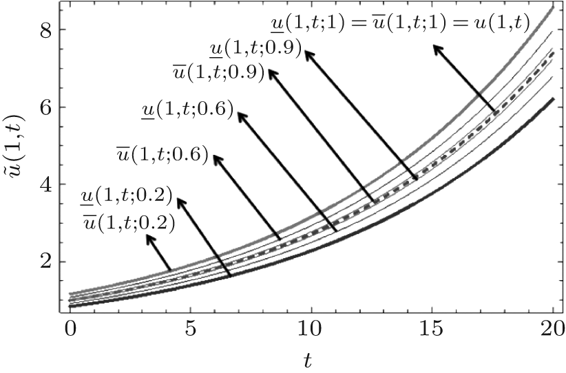	Fig.  5. Interval solutions for Example 2.

Fig.  6.

	Figure Option ViewDownloadNew Window
	Fig.  6. Interval solutions for Example 1 at t = 1.

Fig.  7.

	Figure Option ViewDownloadNew Window
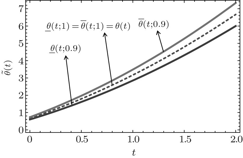	Fig.  7. Interval solutions of uncertain temperature on boundary Γ 2 for Example 1 at r = 0.9.

Fig.  8.

	Figure Option ViewDownloadNew Window
	Fig.  8. Interval solutions of uncertain temperature on boundary Γ 2 for Example 2 at r = 0.9.

Fig.  9.

	Figure Option ViewDownloadNew Window
	Fig.  9. Interval solutions of uncertain heat flux on boundary Γ 2 for Example 1 at r = 0.9.

Fig.  10.

	Figure Option ViewDownloadNew Window
	Fig.  10. Interval solutions of uncertain heat flux on boundary Γ 2 for Example 2 at r = 0.9.

The computed results in digital form for both the examples are also shown in Tables  1 and 3, respectively, by varying x from 0 to 5 and taking t = 1 with r = 0.3. Similar results are tabulated in Tables  2 and 4, respectively, by varying t from 0 to 5 and taking x = 1 with r = 0.3. Also Tables  5 and 6 contains the numerical results for uncertain temperature on boundary Γ ₂ for both the examples for r = 0.6. Similarly, Tables  7 and 8 tabulate the obtained results of uncertain heat flux for r = 0.8. It is interesting to note that in the special case for r = 1, the results exactly match with Hetmaniok et al.^[1] and Bede^[37] with HPM. However, in the Bede method, ^[37] it requires more computation time because we may have to convert the fuzzy differential equations to a system of differential equations depending on the sign of the coefficient.

Table 1.

Table 1.

Table 1. Comparison of present, Bede[37] with HPM, and Hetmaniok et al.[1] solutions of Example 1 with t = 1. x u3(x, t)   Present Ref.  [37] Present Ref.  [37] Presen Ref.  [37] Ref.  [1] 0 0.15 0.15 0.85 0.85 0.5 0.5 0.5 0.5 0.188281 0.188281 1.0669 1.0669 0.627604 0.627604 0.627604 1 0.3125 0.3125 1.7708 1.7708 1.0416 1.0416 1.0416 1.5 0.550781 0.550781 3.1210 3.1210 1.8359 1.8359 1.8359 2 0.95 0.95 5.3833 5.3833 3.1666 3.1666 3.1666 2.5 1.5757 1.5757 8.9294 8.9294 5.2526 5.2526 5.2526 3 2.5125 2.5125 14.237 14.237 8.37 8.37 8.37 3.5 3.8632 3.8632 21.891 21.891 12.877 12.877 12.877 4 5.75 5.75 32.583 32.583 19.166 19.166 19.166 4.5 8.3132 8.3132 47.108 47.108 27.710 27.710 27.710 5 11.712 11.712 66.370 66.370 39.041 39.041 39.041

Table 1. Comparison of present, Bede[37] with HPM, and Hetmaniok et al.[1] solutions of Example 1 with t = 1.

Table 2.

Table 2.

Table 2. Comparison of present, Bede[37] with HPM and Hetmaniok et al.[1] solutions of Example 1 for x = 1 and r = 0.3. t ū 3(x, t) u3(x, t)   Present Ref.  [37] Present Ref.  [37] Present Ref.  [37] Ref.  [1] 0 0.0125 0.0125 0.0708333 0.0416667 0.0416667 0.0416667 0.0416667 0.5 0.125 0.125 0.708333 0.416667 0.416667 0.416667 0.416667 1 0.3125 0.3125 1.77083 1.04167 1.04167 1.04167 1.04167 1.5 0.575 0.575 3.25833 1.91667 1.91667 1.91667 1.91667 2 0.9125 0.9125 5.17083 3.04167 3.04167 3.04167 3.04167 2.5 1.325 1.325 7.50833 4.41667 4.41667 4.41667 4.41667 3 1.8125 1.8125 10.2708 6.04167 6.04167 6.04167 6.04167 3.5 2.375 2.375 13.4583 7.91667 7.91667 7.91667 7.91667 4 3.0125 3.0125 17.0708 10.0417 10.0417 10.0417 10.0417 4.5 3.725 3.725 21.1083 12.4167 12.4167 12.4167 12.4167 5 4.5125 4.5125 25.5708 15.0417 15.0417 15.0417 15.0417

Table 2. Comparison of present, Bede[37] with HPM and Hetmaniok et al.[1] solutions of Example 1 for x = 1 and r = 0.3.

Table 3.

Table 3.

Table 3. Comparison of present, Bede[37] with HPM, and Hetmaniok et al.[1] solutions of Example 2 for t = 1 and r = 0.5. x ū 3(x, t) u3(x, t)   Present Ref.  [37] Present Ref.  [37] Present Ref.  [37] Ref.  [1] 0 2.58358 2.58358 3.42475 3.42475 3.00417 3.00417 3.00417 0.5 1.56702 1.56702 2.07722 2.07722 1.82212 1.82212 1.82212 1 0.950447 0.950447 1.25989 1.25989 1.10517 1.10517 1.10517 1.5 0.576475 0.576475 0.764165 0.764165 0.67032 0.67032 0.67032 2 0.34965 0.34965 0.463489 0.463489 0.40657 0.40657 0.40657 2.5 0.212073 0.212073 0.281121 0.281121 0.246597 0.246597 0.246597 3 0.128629 0.128629 0.170508 0.170508 0.149569 0.149569 0.149569 3.5 0.0780174 0.0780174 0.103418 0.103418 0.090718 0.090718 0.090718 4 0.04732 0.04732 0.0627265 0.0627265 0.0550232 0.0550232 0.0550232 4.5 0.028701 0.028701 0.0380455 0.0380455 0.0333733 0.0333733 0.0333733 5 0.017408 0.017408 0.0230758 0.0230758 0.0202419 0.0202419 0.0202419

Table 3. Comparison of present, Bede[37] with HPM, and Hetmaniok et al.[1] solutions of Example 2 for t = 1 and r = 0.5.

Table 4.

Table 4.

Table 4. Comparison of present, Bede[37] with HPM, and Hetmaniok et al.[1] solutions of Example 2 for x = 1 and r = 0.5. t ū 3(x, t) u3(x, t)   Present Ref.  [37] Present Ref.  [37] Present Ref.  [37] Ref.  [1] 0 0.86 0.86 1.14 1.14 1 1 1 0.5 0.904093 0.904093 1.19845 1.19845 1.05127 1.05127 1.05127 1 0.950447 0.950447 1.25989 1.25989 1.10517 1.10517 1.10517 1.5 0.999177 0.999177 1.32449 1.32449 1.16183 1.16183 1.16183 2 1.05041 1.05041 1.3924 1.3924 1.2214 1.2214 1.2214 2.5 1.10426 1.10426 1.46379 1.46379 1.28403 1.28403 1.28403 3 1.16088 1.16088 1.53884 1.53884 1.34986 1.34986 1.34986 3.5 1.2204 1.2204 1.61774 1.61774 1.41907 1.41907 1.41907 4 1.28297 1.28297 1.70068 1.70068 1.49182 1.49182 1.49182 4.5 1.34875 1.34875 1.78788 1.78788 1.56831 1.56831 1.56831 5 1.4179 1.4179 1.87954 1.87954 1.64872 1.64872 1.64872

Table 4. Comparison of present, Bede[37] with HPM, and Hetmaniok et al.[1] solutions of Example 2 for x = 1 and r = 0.5.

Table 5.

Table 5.

Table 5. Comparison results for uncertain temperature of present, Bede[37] with HPM, and Hetmaniok et al.[1] of Example 1 for r = 0.6. t θ (t)   Present Ref.  [37] Present Ref.  [37] Present Ref.  [37] Ref.  [1] 0.2 0.652 0.652 1.52133 1.52133 1.08667 1.08667 1.08667 0.4 0.928 0.928 2.16533 2.16533 1.54667 1.54667 1.54667 0.6 1.228 1.228 2.86533 2.86533 2.04667 2.04667 2.04667 0.8 1.552 1.552 3.62133 3.62133 2.58667 2.58667 2.58667 1 1.9 1.9 4.43333 4.43333 3.16667 3.16667 3.16667 1.2 2.272 2.272 5.30133 5.30133 3.78667 3.78667 3.78667 1.4 2.668 2.668 6.22533 6.22533 4.44667 4.44667 4.44667 1.6 3.088 3.088 7.20533 7.20533 5.14667 5.14667 5.14667 1.8 3.532 3.532 8.24133 8.24133 5.88667 5.88667 5.88667 2 4 4 9.33333 9.33333 6.66667 6.66667 6.66667

Table 5. Comparison results for uncertain temperature of present, Bede[37] with HPM, and Hetmaniok et al.[1] of Example 1 for r = 0.6.

Table 6.

Table 6.

Table 6. Comparison results for uncertain temperature of present, Bede[37] with HPM, and Hetmaniok et al.[1] of Example 2 for r = 0.6. t θ (t)   Present Ref.  [37] Present Ref.  [37] Present Ref.  [37] Ref.  [1] 0.2 0.768449 0.768449 0.902092 0.902092 0.83527 0.83527 0.83527 0.4 0.783972 0.783972 0.920315 0.920315 0.852144 0.852144 0.852144 0.6 0.79981 0.79981 0.938907 0.938907 0.869358 0.869358 0.869358 0.8 0.815967 0.815967 0.957874 0.957874 0.88692 0.88692 0.88692 1 0.83245 0.83245 0.977224 0.977224 0.904837 0.904837 0.904837 1.2 0.849267 0.849267 0.996966 0.996966 0.923116 0.923116 0.923116 1.4 0.866423 0.866423 1.01711 1.01711 0.941765 0.941765 0.941765 1.6 0.883926 0.883926 1.03765 1.03765 0.960789 0.960789 0.960789 1.8 0.901783 0.901783 1.05861 1.05861 0.980199 0.980199 0.980199 2 0.92 0.92 1.08 1.08 1 1 1

Table 6. Comparison results for uncertain temperature of present, Bede[37] with HPM, and Hetmaniok et al.[1] of Example 2 for r = 0.6.

Table 7.

Table 7.

Table 7. Comparison results for uncertain heat flux of present, Bede[37] with HPM, and Hetmaniok et al.[1] of Example 1 for r = 0.8. t q(t)   Present Ref.  [37] Present Ref.  [37] Present Ref.  [37] Ref.  [1] 0.2 – 1.38667 – 1.38667 – 2.08 – 2.08 – 1.73333 – 1.73333 – 1.73333 0.4 – 1.70667 – 1.70667 – 2.56 – 2.56 – 2.13333 – 2.13333 – 2.13333 0.6 – 2.02667 – 2.02667 – 3.04 – 3.04 – 2.53333 – 2.53333 – 2.53333 0.8 – 2.34667 – 2.34667 – 3.52 – 3.52 – 2.93333 – 2.93333 – 2.93333 1 – 2.66667 – 2.66667 – 4 – 4 – 3.33333 – 3.33333 – 3.33333 1.2 – 2.98667 – 2.98667 – 4.48 – 4.48 – 3.73333 – 3.73333 – 3.73333 1.4 – 3.30667 – 3.30667 – 4.96 – 4.96 – 4.13333 – 4.13333 – 4.13333 1.6 – 3.62667 – 3.62667 – 5.44 – 5.44 – 4.53333 – 4.53333 – 4.53333 1.8 – 3.94667 – 3.94667 – 5.92 – 5.92 – 4.93333 – 4.93333 – 4.93333 2 – 4.26667 – 4.26667 – 6.4 – 6.4 – 5.33333 – 5.33333 – 5.33333

Table 7. Comparison results for uncertain heat flux of present, Bede[37] with HPM, and Hetmaniok et al.[1] of Example 1 for r = 0.8.

Table 8.

Table 8.

Table 8. Comparison results for uncertain heat flux of present, Bede[37] with HPM, and Hetmaniok et al.[1] of Example 2 for r = 0.8. t q(t)   Present Ref.  [37] Present Ref.  [37] Present Ref.  [37] Ref.  [1] 0.2 1.60372 1.60372 1.73736 1.73736 1.67054 1.67054 1.67054 0.4 1.63612 1.63612 1.77246 1.77246 1.70429 1.70429 1.70429 0.6 1.66917 1.66917 1.80827 1.80827 1.73872 1.73872 1.73872 0.8 1.70289 1.70289 1.84479 1.84479 1.77384 1.77384 1.77384 1 1.73729 1.73729 1.88206 1.88206 1.80967 1.80967 1.80967 1.2 1.77238 1.77238 1.92008 1.92008 1.84623 1.84623 1.84623 1.4 1.80819 1.80819 1.95887 1.95887 1.88353 1.88353 1.88353 1.6 1.84472 1.84472 1.99844 1.99844 1.92158 1.92158 1.92158 1.8 1.88198 1.88198 2.03881 2.03881 1.9604 1.9604 1.9604 2 1.92 1.92 2.08 2.08 2 2 2

Table 8. Comparison results for uncertain heat flux of present, Bede[37] with HPM, and Hetmaniok et al.[1] of Example 2 for r = 0.8.

In this paper the double parametric form of fuzzy numbers has successfully been applied to the solution of an uncertain inverse heat conduction problem using the variational iteration method (VIM). The double parametric form approach is found to be easy and straight forward. The double parametric form approach is easy and straightforward. This does not change the order of original fuzzy differential equations. However, Bede^[37] in his method converted the fuzzy differential equations to two crisp differential equations or system of differential equations depending on the sign of the coefficients. Hence, it takes more time than the present method, which is a double parametric form of fuzzy number. Here, the performance of the method has been shown by using the initial condition as the triangular fuzzy number. Firstly, the uncertain temperature distribution in the domain is computed. Then, reconstruction of functions describing the uncertain temperature and heat flux on the boundary has been done when uncertain temperature measurement is known. It is interesting to note for r = 1 in both the examples that the lower and upper uncertain temperature distributions are equal. From the results, one may conclude that the HPM and VIM can be used as alternative and equivalent methods for obtaining analytical and approximate solutions of forward and inverse heat conduction problems because the solution takes the form of a convergent series with easily computable components.