


Retrieval of original signals for superconducting quantum interference device operating in flux locked mode
[Liu Dang-Ting, Tian Ye† , Zhao Shi-Ping, Ren Yu-Feng, Chen Geng-Hua]
, Zhao Shi-Ping, Ren Yu-Feng, Chen Geng-Hua]
|
|


†Corresponding author. E-mail: yetian@aphy.iphy.ac.cn
We discuss a simple relation between the input and output signals of a superconducting quantum interference device magnetometer operating in flux locked mode in a cosine curve approximation. According to this relation, an original fast input signal can be easily retrieved from its distorted output response. This technique can be used in some areas such as sensitive and fast detection of magnetic or metallic grains in medicine and food security checking.
The superconducting quantum interference devices (SQUIDs) have been widely used as extremely sensitive magnetic sensors in many fields for decades.[1– 9] Their performance improvements[10, 11] and applications in various interesting new areas such as superconducting quantum computation[12– 14] have continued to attract much attention today. SQUID magnetometers may operate in two different modes, namely, the flux locked (closed loop) and unlocked modes (open loop).[3] In the unlocked mode, they usually have very high speed in response to the input flux change, but poor linearity and dynamic range. On the other hand, in the flux locked mode, by using SQUID as a null detector of flux, the transfer function is linearized. In this case, the SQUID magnetometers have both good linearity and dynamic range, but somewhat lower response speed due to the feedback mechanism. The feedback also causes a signal distortion, which is sometimes unnoticed in applications where the signal does not vary rapidly.
The output flux of a SQUID magnetometer operating in a flux locked mode is not always equal to the input signal, except in the case of static input. The working point for a static input is at one of the maxima or minima of transfer function V(Φ ), where dV/dΦ = 0. If we assume that the input flux rises up or falls down at a constant speed, namely, dΦ in/dt = constant, it will cause a shift of the working point from the static position and furthermore have a finite slope dV/dΦ ≠ 0. With a flux modulation, the phase detector and integrator produce an increasing/decreasing feedback flux to track the input flux. As soon as the feedback flux rate reaches the input flux rate, a balance state is established, and the balance working point is set to be at Φ out with a flux shift of Δ Φ . For a slowly varying input signal, the flux shift Δ Φ is negligible and the feedback flux (output signal) can be regarded as an input flux. However, when the input signal changes very fast (but still smaller than the through rate), the instantaneous flux shift could be as large as Δ Φ ≈ ± Φ 0/4 (Φ 0 = h/2e ≈ 2.07 × 10− 15 Wb is flux quantum), and the original signal is distorted seriously. This can cause problems in some applications, such as fast detection of magnetic or metallic grains for medicine and food security checking.
In this paper we discuss a simple relation between the input and output signals of a flux locked SQUID magnetometer in a cosine curve approximation. According to this relation, the original input signals can be easily retrieved from the distorted output waveforms.
The flux-to-voltage transfer function V(Φ ) of both dc- and rf-SQUID has strongly nonlinear periodic behavior. Nevertheless, it can be well approximated by a function with cosine curve (see Fig. 1) as

where c is determined by the bias current of a SQUID.
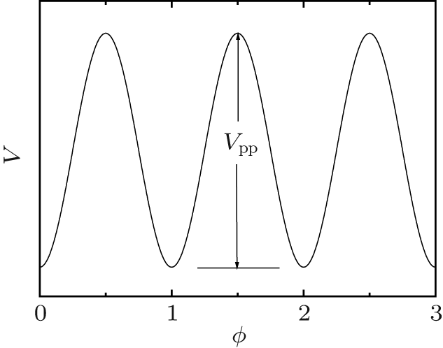 | Fig. 1. Transfer function V(Φ /Φ 0) approximated by a cosine curve. |
In the flux locked mode, the SQUID works around one of the maxima or minima of the transfer function. Without losing generality, we assume that the static working point is a minimum at Φ = 0, where the feedback flux does not change with time except noise. As soon as a flux displacement Δ Φ occurs, the feedback flux obtains an increasing rate (or a decreasing rate). The rate reaches its maximum value at Δ Φ = ± Φ 0/4, which is called through rate R. An input flux whose increasing rate (or decreasing rate) exceeds the through rate may not be well locked.
In the cosine curve approximation, the transfer coefficient dV/dΦ at Φ = Δ Φ is

For small Δ Φ , dV/dΦ can be expressed in the first approximation as

Since the rate of feedback flux is directly proportional to dV/dΦ , it can be written as

in a range of | Δ Φ | ≤ Φ 0/4. At Δ Φ = Φ 0/4, tracking velocity is largest and equal to through rate R, so γ = 4R/Φ 0. As noted above, the displacement of the flux Δ Φ represents the difference between input flux Φ in and output (feedback) flux Φ out, namely

In the dimensionless unit, we define

Combining Eqs. (4), (5), and (6), we have

For a given input signal ϕ in(τ ), we may obtain the response output ϕ out(τ ) by solving the above equation and it can be shown

where D ≡ d/dτ is ordinary differential operator, and ϕ out(0) and ϕ in(0) represent the values of ϕ out(τ ) and ϕ in(τ ) at τ = 0, respectively. Equation (8) indicates that the function of the initial condition will fade out after a long time τ ≫ 1.
As an example, we assume that the input signal is a step function

From Eq. (8), we obtain the output response

or

which depends on the initial condition output flux Φ out(0). Both ϕ in(τ ) and ϕ out(τ ) are depicted in Fig. 2. It shows that the output response to the input signal has a time delay, so it is distorted.
 | Fig. 2. Different forms of ϕ out(τ ) acquired from the same ϕ in(τ ) because of different values of ϕ out(0). |
Another example is the sinusoidal input signal as depicted in Fig. 3(a) with the initial condition ϕ out(0) = 0, where Ω = ω Φ 0/4R is the frequency in the dimensionless unit:

From Eq. (8), we obtain

where ϕ = arctanΩ = arctan(ω ϕ 0/4R). The output response ϕ out(τ ) (depicted in Fig. 3(a), where Ω = π /2) shows the distortion of the sinusoidal signal. The dependences of phase shift ϕ and amplitude (1 + Ω 2)− 1/2 of the output signal on frequency are shown in Figs. 3(b) and 3(c) respectively, from which we can draw the following conclusions: in the limit Ω ≫ 0, where the frequency of input signal ω ≫ 0 or the through rate of SQUID magnetometer R → 0, the lag phase of the output signal tends to π /2 and the amplitude to 0; while in the case of Ω → 0, where ω → 0 or R ≫ 0, the phase and amplitude of the output signal are almost the same as those of the input signal.
 | Fig. 3. (a) Input (solid line) and output (dashed line) signals versus time, (b) the dependence of the phase shift of the output response on frequency, and (c) relation between the amplitude and frequency of the output signal. |
In magnetocardiography (MCG) experiments, the data acquisition is carried out by using two SQUID sensors immersed in liquid nitrogen or liquid helium, a pickup SQUID for the signal channel, and a compensatory one for the reference channel. The filtering algorithms, such as gradiometer and adaptive filtering, [15– 18] are used to eliminate environmental noises. However, with the same input signal, the output responses of the two SQUID magnetometers are different because of different through rates, and then the filtering efficacies of these schemes for the output response are weakened. So these filtering schemes must be used in the input signal, which can be retrieved from the output response with calibrated through rate, in order to have more powerful noise suppression.
As the last example, the input signal is described by two consecutive Gaussian functions with variance σ 2 = 0.5 and the same peak height, and the centers of their peaks are Δ τ apart. Figures 4(a) and 4(b) respectively show the input and output signals each with a difference of Δ τ .
 | Fig. 4. (a) Input (solid line) and output (dashed line) signals, each with Δ τ = 2, versus time, and (b) input (solid line) and output (dashed line) signals versus time, the input signal with Δ τ = 1.2 has two obvious peaks, while the output signal has two undistinguishable peaks. |
From Figs. 4(a) and 4(b), we can see that only one peak exists in the output response when the time interval of the two consecutive Gaussian functions is too short. In medicine and food security checking, the exact number of magnetic grains can be found from the input signal, which can be easily retrieved from the output signal.
In the measurement, the original signals ϕ in(τ ) can be easily obtained by using Eq. (7), and it is uniquely determined by the output response. With ϕ out(τ ), the equation can be written as

On the left-hand side of Eq. (14), there are two terms containing Φ out(t) and dΦ out(t)/dt, which reflect the static contribution and the dynamic response, respectively. Before retrieval, the through rate R in flux locked mode should be calibrated.
Now, we show two examples in Figs. 5 and 6 respectively. The response function in Fig. 5 is expressed as

where r is a constant. The original signal can be computed according to Eq. (14), and ϕ in(τ ) turns out to be a linear function of time with a slope of r, i.e.,

The flux shift is Δ ϕ = r − re− τ , which has ϕ = r as an asymptote when τ tends to + ∞ , and it reduces to zero at τ = 0. The signal can be kept to be locked when | Δ ϕ | ≤ 1/4 (the equal sign holds only when noise is not present). It can be shown that the locking condition is ϕ in(τ ) = rτ < τ /4 (or Φ in(t) < Rt) since r < 1/4.
 | Fig. 5. Input signal expressed by a linear function of τ with slope r = 1/8 and the output response. |
 | Fig. 6. Original signal (solid line) and output response (dashed line). |
In Fig. 6, the response function is

where k is a twentyfold integer. Using Eq. (14), we obtain the original waveform

The original signal is a square wave function, whose varying rate is nonzero only at the points of the decuple integer, and the locking condition is | β | < 1/4.
In this paper, we discuss an effective way to retrieve rapidly varying original signals in the SQUID magnetometer applications. With V(Φ ) approximated by a cosine function, the relation between the input signal and the output signal is obtained analytically. We show that the retrieved input signal depends not only on the output signal but also on its change. Using this relation, we can find the original signal conveniently from the output response.
We thank Q. S. Yang and L. H. Zhang for many helpful discussions during this work.
| 1 |
|
| 2 |
|
| 3 |
|
| 4 |
|
| 5 |
|
| 6 |
|
| 7 |
|
| 8 |
|
| 9 |
|
| 10 |
|
| 11 |
|
| 12 |
|
| 13 |
|
| 14 |
|
| 15 |
|
| 16 |
|
| 17 |
|
| 18 |
|