
Thermal and thermoelectric response from Keldysh formalism with application to gapped Dirac fermions*
[Zhu Guo-Baoa), b)†  , Yang Hui-Min
a) , Yang Sheng-Yuanc) ]
, Yang Hui-Min|
|


†Corresponding author. E-mail: zhuguobao@gmail.com
*Project supported by the Special Funds of the National Natural Science Foundation of China (Grant No. 11447145) and the Doctoral Program of Heze University, Shandong Province, China (Grant No. XY14B002).
Based on the Keldysh Green’s functions theory, we present a general formula of the thermal and thermoelectric transport. In the clean limit, our formula recovers the previous results obtained from the semiclassical transport theory. In our approach, we propose an appropriate energy current operator and electric current operator, and the unphysical divergence from the direct application of the Kubo formula is eliminated. As an application, we study the thermal and the thermoelectric Hall conductivities of a gapped Dirac fermion model in the presence of impurity scattering.
The study of energy transport in various systems has attracted a lot of attention.[1– 4] The control of the heat fluxes and minimization of the related energy loss are important factors in modern electronics. Energy transport in metals or semiconductors is mainly related to the electric current flow. Electrons move in the materials, carrying not only charge but also energy. A temperature gradient can generate both electric current and energy (heat) current. In linear response, the electric and thermal transport induced by a temperature gradient is given by the following relation

where je and jE represent the electric and heat current densities, respectively. 

Transport properties can be affected by electrical, optical, and magnetic means. The corresponding mechanical force on the carriers are the electric force and the Lorentz force; however, there is no mechanical force that corresponds to the temperature gradient. Therefore, many of the theoretical tools which are used to describe charge (spin) transport cannot be straightforwardly extended to the study of heat transport. The direct application of linear response theory typically yields unphysical divergence[5– 7] at zero temperature. In this paper, by choosing an appropriate energy operator and electric current operator with auxiliary gravitational field we are able to derive general formulas for the thermal and thermoelectric conductivities based on the Keldysh Green functions theory.[8– 16] The method can eliminate the troublesome divergence from the direct application of the Kubo formula. We show that in the clean limit, our formula reduces to the previous results obtained from other approaches. Expressed in terms of Green’ s function, our result has the advantage that disorder effects and interaction effects can be systematically studied using the standard perturbation method. As an application, we study the thermal and thermoelectric Hall conductivities in a disordered gapped Dirac model.
The structure of this paper is organized as follows. In Section 2 we derive our general formula of thermal and thermoelectric conductivities. In Section 3, we present the application of our formula to study the thermal and thermoelectric Hall conductivities in the disordered gapped Dirac fermion model. In Section 4, we summarize our results.
In this section, we derive the thermal and thermoelectric transport coefficients in the presence of the temperature gradient in the linear response regime. However, it is not possible to directly incorporate the temperature gradient into the Hamiltonian as an external field. This is because the temperature gradient is a statistical force that affects the particles through the distribution function rather than a dynamical force that exerts direct force to the particle. To solve this problem, Luttinger[17] proposed a method to study first the response due to the mechanic force from an inhomogenous gravitational field, then using the Einstein relation to relate the obtained transport coefficients to the thermal transport coefficients.
We follow Luttinger’ s method, and introduce an auxiliary gravitational field γ to the Hamiltonian. In the presence of gravitational field γ corresponding to the mechanic counterpart of the temperature gradient, the term in Hamiltonian due to the interaction with this field[9] is

We note that by including the interaction, the velocity operator becomes

and the energy current operator becomes

where 


where lesser Green’ s function Ĝ < (ε , k) can be determined by introducing the auxiliary gravitational field γ into the Dyson equation. The Dyson equation for Green’ s function in the presence of Luttinger’ s gravitational field γ (r) is
where Ĝ (r, t; r′ , t′ ) = − i 〈 Tc{ψ (r, t)ψ † (r′ , t′ )}〉 is the contour-ordered Green’ s function matrix, and 

Where nimp and Vimp denote a possible disorder concentration and potential respectively. By applying the following transformation to the Dyson equation (7)

with 

After Fourier transforming the relative time, the Dyson equation in the linear response regime becomes

Here we separated the dependence on the center of mass and the relative coordinates. Then, we have the ∇ γ -dependent part of the Green function given by
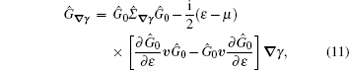
where Ĝ ∇ γ and 


Using the above relations, we can separate G< into two terms: a Fermi surface contribution and a Fermi sea contribution

where
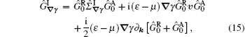

and
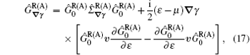

First we consider the simplest clean limit result. This also serves as a check of our theory. In this case, the retarded and advanced Green’ s functions are just given by

Ĥ 0 is disorder free part of the Hamiltonian. Plugging Eq. (19) into Eq. (6), we can obtain

Using the residue theorem, we find that

After some algebra (the same procedure described in Refs. [9] and [10]), we obtain
Here 

In the following we apply our derived formula to study the thermal and thermoelectric Hall conductivities of the 2D gapped Dirac model. This model has been widely used to describe systems such as gapped graphene and gapped topological insulator surfaces.[19, 20] It can be written as

where 


the corresponding wave functions are

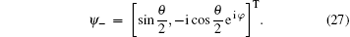
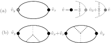
Where φ = arctan(ky/kx) is the azimuthal angle (see Fig. 1),

is the polar angle (see Fig. 1), and we have unitized the size of the system.
 | Fig. 1. Schematic diagram for azimuthal angle φ and polar angle θ . |
In the following we consider that the system is electron doped with ε F > Δ . Due to particle hole symmetry, the results can be easily generalized to the hole-doped case. In our model, we assume that the impurities are dilute, and then we obtain the self-energy using Born approximation[21]
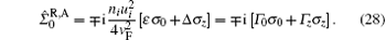
Since we have assumed that 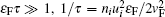


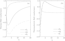
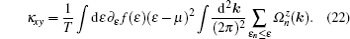
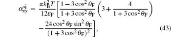
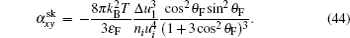
where the first term denotes an intrinsic Berry curvature-driven contribution, and the other two terms caused by the scattering of electrons off impurities: the side-jump contribution and the skew-scattering contribution.[23] According to the diagrammatic representation as shown in Fig. 2, the side-jump contribution and skew-scattering contribution to thermal and thermoelectric conductivity are
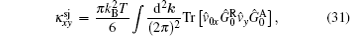

and
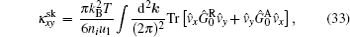
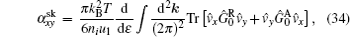
respectively. Where

is the ladder-diagram corrected velocity vertex, 

 | Fig. 2. Graphical representation (a) of the side-jump contribution and (b) of the skew-scattering contribution. The solid lines are the disorder averaged Green’ s functions, and the dashed lines with crosses represent disorder scattering. |
When ε F > Δ , the intrinsic contributions (above band gap) can be calculated by Eqs. (22) and (23) using Sommerfeld expansion, and we have

Straightforward calculations show that


Where


and
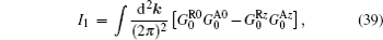
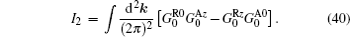


when both subbands are partially occupied, i.e., ε F > Δ , where sinθ F = γ kF/ε F. Then we obtain


and
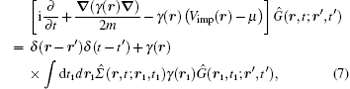
The skew scattering contribution only dominates in the ultraclean limit.[22] Here we are most interested in the sum of intrinsic and side-jump thermal 


can be obtained from anomalous Hall conductivity[22, 23] based on Wiedemann– Franz law. The thermoelectric Hall conductivity

can be obtained from anomalous Hall conductivity based on the Mott rule. The calculations here again demonstrate the validity of our formula.
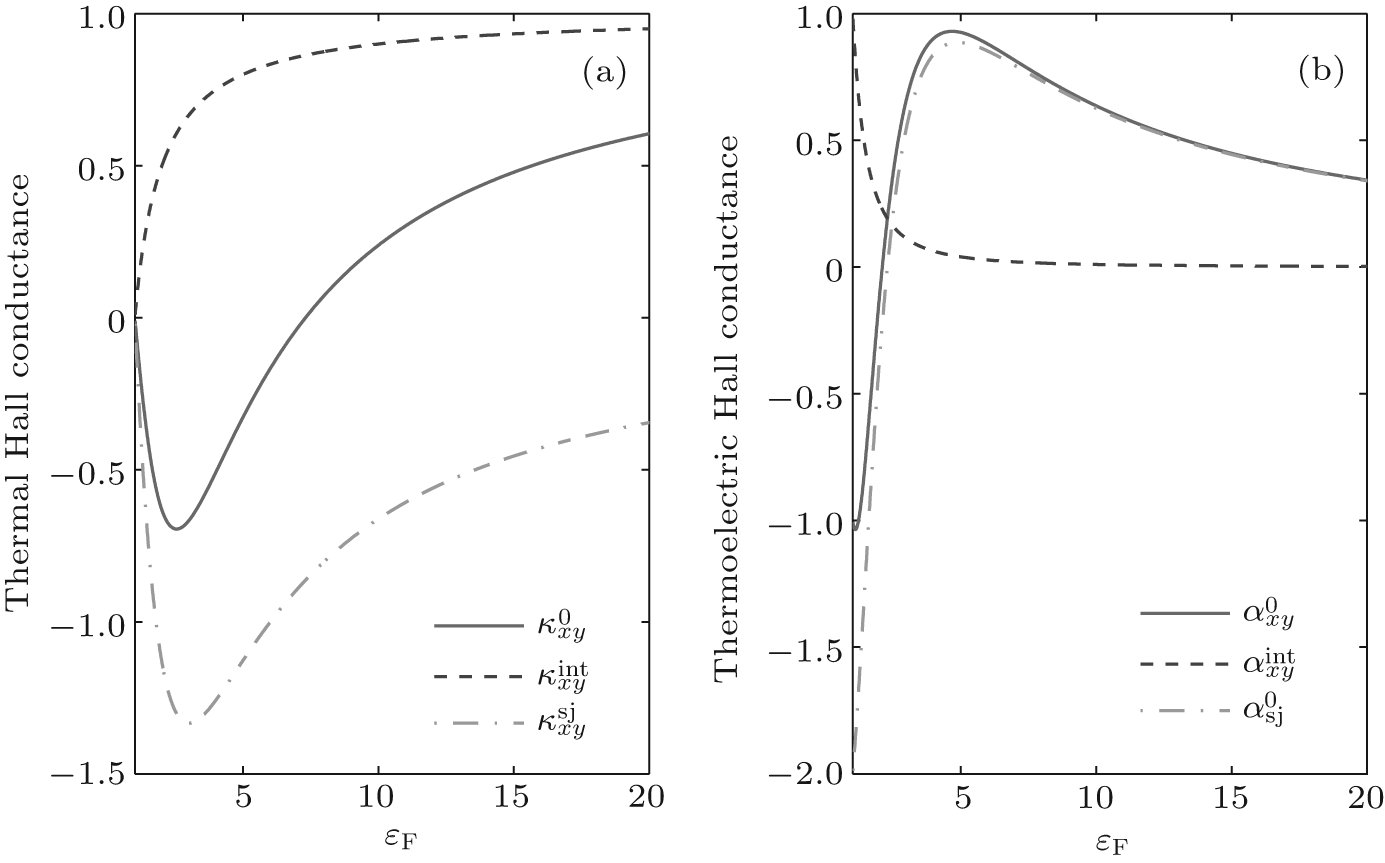 | Fig. 3. The intrinsic contribution (dashed blue curve), side-jump contribution (dash-dotted green curve), and their sum (solid red curve) to thermal Hall conductivity (a), and thermoelectric Hall conductivity (b) as a function of the Fermi energy ε F. The thermal Hall conductivity is measured in units of   |
In summary, we have derived a general formula of the thermal and thermoelectric transport of disordered electron systems based on the Keldysh Green’ s functions theory. Following the method proposed by Luttinger, we proposed an appropriate energy current operator and electric current operator. The unphysical divergence from the direct application of the Kubo formula is eliminated in our approach. In the absence of disorders, our formula recovers the previous results obtained from the semiclassical theory. As an application, we studied extrinsic thermal and thermoelectric Hall conductivities of a disordered gapped Dirac model. Our theory would be useful for systematic studies of disorder and interaction effects in thermal transport phenomena.
| 1 |
|
| 2 |
|
| 3 |
|
| 4 |
|
| 5 |
|
| 6 |
|
| 7 |
|
| 8 |
|
| 9 |
|
| 10 |
|
| 11 |
|
| 12 |
|
| 13 |
|
| 14 |
|
| 15 |
|
| 16 |
|
| 17 |
|
| 18 |
|
| 19 |
|
| 20 |
|
| 21 |
|
| 22 |
|
| 23 |
|
| 24 |
|