

Experimental verification of effect of horizontal inhomogeneity of evaporation duct on electromagnetic wave propagation*
[Shi Yang, Yang Kun-De† , Yang Yi-Xin, Ma Yuan-Liang]
, Yang Yi-Xin, Ma Yuan-Liang]
|
|


†Corresponding author. E-mail: ykdzym@nwpu.edu.cn
*Project supported by the National Natural Science Foundation of China (Grant No. 11174235) and the Fundamental Research Funds for the Central Universities (Grant No. 3102014JC02010301).
The evaporation duct which forms above the ocean surface has a significant influence on electromagnetic wave propagation above 2 GHz over the ocean. The effects of horizontal inhomogeneity of evaporation duct on electromagnetic wave propagation are investigated, both in numerical simulation and experimental observation methods, in this paper. Firstly, the features of the horizontal inhomogeneity of the evaporation duct are discussed. Then, two typical inhomogeneous cases are simulated and compared with the homogeneous case. The result shows that path loss is significantly higher than that in the homogeneous case when the evaporation duct height (EDH) at the receiver is lower than that at the transmitter. It is also concluded that the horizontal inhomogeneity of the evaporation duct has a significant influence when the EDH is low or when the electromagnetic wave frequency is lower than 13 GHz. Finally, experimental data collected on a 149-km long propagation path in the South China Sea in 2013 are used to verify the conclusion. The experimental results are consistent with the simulation results. The horizontal inhomogeneity of evaporation duct should be considered when modeling electromagnetic wave propagation over the ocean.
Humidity decreases rapidly in the atmospheric surface layer (ASL) above the ocean surface, resulting in a leaky wave guide which bends electromagnetic wave propagation towards the ocean surface. This feature is known as the evaporation duct, which has a significant influence on electromagnetic wave propagation along the low-altitude path above 2 GHz over the ocean. The evaporation duct almost exists over all of the world' s oceans and it usually affects the performance of low-altitude radar and communication systems.[1– 4]
Numerous propagation models have been developed to simulate electromagnetic wave propagation in the troposphere, such as ray optics model, parabolic equation model, [5– 8] waveguide mode model, [9] and hybrid model.[10] The advanced propagation model (APM) is a hybrid model which combines radio physical optics (RPO) and terrain parabolic equation model (TPEM). The APM model accounts for terrain and rough sea surface effects along the propagation path. It is believed to be accurate and used in the advanced refractive effects prediction system (AREPS). However, a large error exists between the model' s results and the experimental results when modeling the electromagnetic wave propagation in an evaporation duct.[3] The range-dependent evaporation duct environment is believed to be an important factor when modeling electromagnetic wave propagation in an evaporation duct, but relevant research has seldom been reported.
Traditional methods, such as direct measurements, [11, 12] inversion methods, [13– 15] and numeral models, [16, 17] cannot provide an inhomogeneous environment on the propagation path. The developments of data assimilation and mesoscale numerical weather prediction (NWP) techniques make it possible to investigate the horizontal inhomogeneity of the evaporation duct. The reanalysis products[18, 19] can supply the long term, high spatial, and temporal resolution atmospheric data near the sea surface, which can be used to calculate a modified refractivity profile in the evaporation duct. For example, the spatial resolution of the National Center for Environmental Prediction (NCEP) Climate Forecast System Reanalysis (CFSR) data[19] is 0.313° × 0.312° (about 30 km) and the temporal resolution is an hour. The NWP model, such as the weather research and forecasting (WRF) model, [20] the Pennsylvania State University/National Center for Atmospheric Research (PSU/NCAR) mesoscale model (known as MM5 model)[21] and the coupled ocean/atmosphere mesoscale prediction system (COAMPS) model[22] can also provide atmospheric data with high spatial and temporal resolution. The WRF model can provide a result with up to 3-km spatial resolution and an hourly temporal resolution forecast. The high spatial and hourly temporal resolution is very valuable to distinguish the diurnal variations in EDH. Based on the data obtained from these assimilation methods and NWP models, the effects of the inhomogeneity of the evaporation duct on electromagnetic wave propagation can be further studied.
The rest of this paper is structured as follows. The features of horizontal inhomogeneity of evaporation duct are discussed in Section 2. The electromagnetic wave propagation in inhomogeneous evaporation duct is simulated in Section 3. By comparing the result with that in the homogeneous case, the effects of horizontal inhomogeneity of evaporation duct on electromagnetic wave propagation are discussed. In Section 4, the evaporation duct experiment held in the South China Sea in 2013 is introduced. The data collected in the experiment is used to verify the conclusion.
The propagations of microwave and millimeter-wave electromagnetic radiation in the atmosphere depend on gradient of the refractivity index of air. The refractive index is the ratio of the speed (c) of an electromagnetic wave in a vacuum to that in the material of interest (v), i.e.,

Since n nearly equals 1 in the troposphere (the typical value is 1.0003), the refractive index is represented by a quantity called the radio refractivity N as

For the electromagnetic wave whose frequency range is from 1 GHz to 100 GHz, the refractivity N can be calculated by the following empirical equation:

where T (in unit K) is the atmospheric temperature, P (in unit hPa) is the total atmospheric pressure, e (in unit hPa) is the water– vapor pressure, and the constants have been empirically determined. Modified refractivity, which takes the earth' s curvature into consideration, is defined as

where z (in unit m) is the altitude above sea level, more information can be found in Babin' s research.[11]
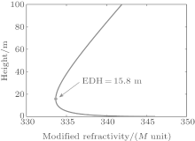
The vertical gradient of M determines the type of refraction conditions: normal, super-refraction or sub-refraction. When the M gradient is positive, sub-refraction occurs and the electromagnetic waves bend upwards. When the M gradient is negative, super-refraction occurs and the propagating electromagnetic waves bend downward. When the evaporation duct occurs, the electromagnetic waves bend downward and reflect from the sea surface in a repeating process. The evaporation duct height is the point where the local minimum M is located near the sea surface. The modified refractivity profile calculated by the Naval Postgraduate School (NPS) model is shown in Fig. 1. The evaporation duct height is 15.8 m.
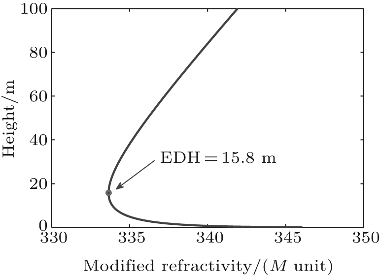 | Fig. 1. Modified refractivity profile (EDH = 15.8 m, air temperature: 20 ° C, sea surface temperature: 20 ° C, relative humidity: 65% , wind speed: 8 m/s, pressure: 1022.2 hPa). |
The EDH is affected by meteorological factors near the sea surface, such as air temperature, relative humidity, wind speed, and sea surface temperature.[16– 19] The uneven distribution of meteorological factors leads to the horizontal inhomogeneity of the evaporation duct. The features of the horizontal inhomogeneity of evaporation duct are discussed as follows.
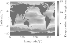
The EDH changes significantly along different latitudes. Figure 2 shows the average EDH over the world’ s ocean in 2008 and figure 3 shows the average EDH along different latitudes. The result is calculated based on the NCEP CFSR product and the Naval Postgraduate School (NPS) model. The details of the method can be found in Ref. [23]. It is shown that the average EDH is about 11 m over the ocean near the equator and the EDH will decrease as the latitude increases from 15° to 50° . As a result, the effect of the horizontal inhomogeneity of the evaporation duct on electromagnetic wave propagation should be considered carefully if the propagation path is along different latitudes.
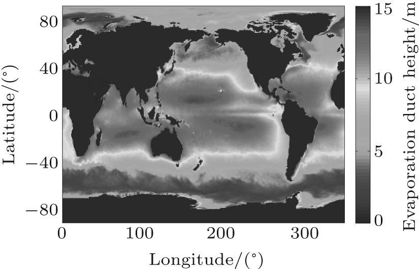 | Fig. 2. Average EDH over the world’ s ocean in 2008. |
 | Fig. 3. Average EDH of world’ s ocean along different latitudes. |
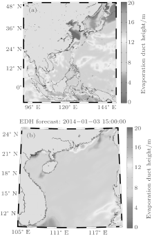
The horizontal inhomogeneity of an evaporation duct is significant in coastal regions. Figure 4(a) shows the EDH reanalysis result in the west Pacific Ocean for 01Z, 1 July 2008. The result is also calculated based on the NCEP CFSR product and the NPS model. It is worth noting that the distribution of EDH is inhomogeneous, especially in the Taiwan Strait, the East China Sea, and the Yellow Sea. For example, the EDH is below 4 m in the Yellow Sea and the north part of the East China Sea. While in the south part of the East China Sea, the EDH is about 15 m. What is more, there are also several areas with high EDH in the South China Sea and the west Pacific Ocean. If the propagation path is located on the edges of these areas or coastal regions, the electromagnetic wave propagation could be influenced by the horizontal inhomogeneity of the evaporation duct.
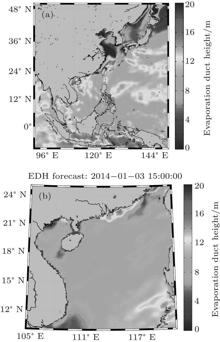 | Fig. 4. (a) Reanalysis result of EDH (unit: m) in the west Pacific Ocean for 01Z, 1 July 2008, and (b) the EDH forecast result in the South China Sea for 15Z, 3 January 2014. |
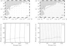
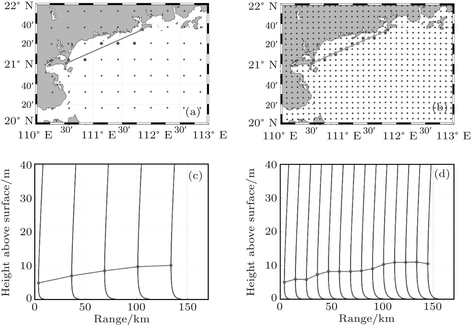 | Fig. 5. Range-dependent modified refractivity profile: (a) the selected points in the first domain (the grid points with circle), (b) the selected points in the second domain (the grid points with circle), (c) modified refractivity profiles of the first domain, and (d) modified refractivity profiles of the second domain. |
There are significant changes of EDH in a span of 30 km. Figure 4(b) shows the EDH forecast result in the South China Sea for 15Z, 3 January 2014. The result is calculated by the WRF model and the NPS model. Figure 5 shows the range-dependent profile extracted from the EDH forecast result for 15Z, 3 January 2014. The propagation path which is 149-km long is located in the north part of the South China Sea near coastal areas, since the evaporation duct experiment was conducted here in 2013. The grid points which are the closest to the propagation path are used to calculate the modified refractivity profile. Figures 5(a) and 5(b) show the selected grid points in the first domain and the second domain of the WRF model, respectively. Since the spatial resolution of the first domain is about 30 km, five modified refractivity profiles are obtained on the propagation path (Fig. 5(c)). Meanwhile, the spatial resolution of the second domain is 10 km and fourteen modified refractivity profiles are obtained on the propagation path (Fig. 5(d)). It can be seen that there are noticeable changes in 30-km intervals and so the profiles provided by the second domain are preferable, if they are available.
The parabolic equation (PE) method has been widely used to calculate electromagnetic wave propagation in the troposphere. The advantage of the PE method is that it can simulate electromagnetic wave propagation in a range-dependent troposphere environment. The standard parabolic equation can be obtained from the Helmholtz equation under certain assumptions and is expressed in the form of

where u represents a scalar component of the electric field for horizontal polarization or a scalar component of the magnetic field for vertical polarization, z is the height, and x is the range, k0 is the free space wave number, and m is the modified refractive index.
Let u(xk, z) be the complex scalar component of the field in a range xk and at height z. Then, the field in a range xk + 1 and at height z, denoted by u(xk + 1, z), could be given by the Fourier split-step solution of PE as

where F[· ] and F− 1[· ] are the Fourier transform and the Fourier inverse transform, respectively, p is the transform variable, and δ x is the range increment, defined as δ x = xk+ 1 − xk. Detailed information about Fourier split-step PE solution can be found in Ref. [24].
In the present paper, the APM[25] is used to calculate the electromagnetic wave propagation in an evaporation duct. APM is a hybrid model which combines radio physical optics (RPO) and terrain parabolic equation model (TPEM) in a relative fast code. The modified refractivity profile is calculated by the NPS model in the numerical simulation.
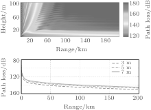
Firstly, the electromagnetic wave propagation in homogenous evaporation duct is calculated and the simulation conditions are shown in Table 1. The propagation path is 200 km and the electromagnetic wave frequency is 10.5 GHz. The EDH is 15 m on the propagation path. Figure 6 shows the electromagnetic wave propagation in a homogeneous evaporation duct. It is shown that the evaporation duct behaves like a waveguide and can lead to a decreased path loss. For example, the path loss is about 140 dB at 50 km when the receiving antenna height is 3 m. The path loss at 200 km is about 150 dB, which is only 10-dB higher than that at 50 km. If the receiving antenna is located outside the evaporation duct, then the path loss is about 20 dB– 30 dB higher than that inside the evaporation duct.
| Table 1. Simulation conditions. |
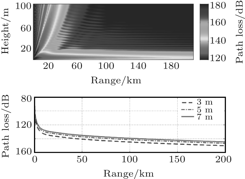 | Fig. 6. Electromagnetic wave propagations in homogeneous evaporation duct. |
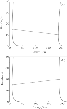
Two cases are then simulated to study the electromagnetic wave propagation in an inhomogeneous evaporation duct. The EDH increases on the propagation path in one case and decreases in the other. The modified refractivity profiles for the two cases are shown in Fig. 7. The EDH at transmitting antenna is 15 m and the EDHs at receiving antenna are 20 m and 10 m, separately.
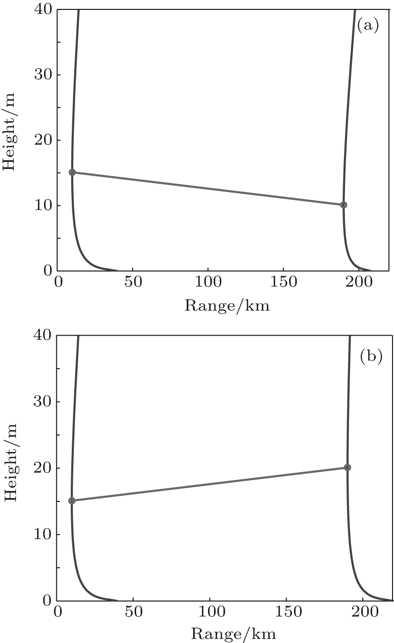 | Fig. 7. Inhomogeneous evaporation ducts: (a) EDH: 15 m– 10 m and (b) EDH: 15 m– 20 m. |
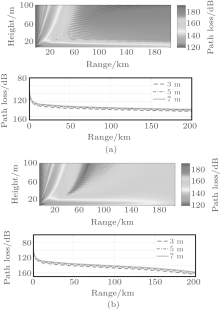
It is shown in Fig. 8 that the electromagnetic wave can be trapped in the two cases. However, their influences on electromagnetic wave propagation are quite different. When the EDH at the receiving antenna is higher than that at the transmitting antenna, the trapping feature of evaporation duct is stronger than that in the opposite case. The path loss is significantly lower in this case. The reasons for this are as follows. In the first case (EDH: 15 m– 20 m), the EDH increases along the propagation path and the trapping feature becomes stronger. The electromagnetic wave which departs from the evaporation duct returns to the duct due to the refractivity. This will reduce the path loss in the evaporation duct. While in the second case (EDH: 15 m– 10 m), the EDH decreases along the propagation path and the trapping feature of the duct becomes weaker. As a result, the electromagnetic wave cannot be trapped and leaves the evaporation duct. Figure 9(a) shows a comparison of path loss at 3 m between in a homogeneous evaporation duct and in an inhomogeneous evaporation duct. The path loss at 200 km in the first case (EDH: 15 m– 20 m) is about 1-dB lower than that in homogeneous case. While the path loss in the second case (EDH: 15 m– 10 m) is about 13-dB higher than that in a homogeneous condition. There is a difference of about 14 dB in path loss between the two inhomogeneous cases.
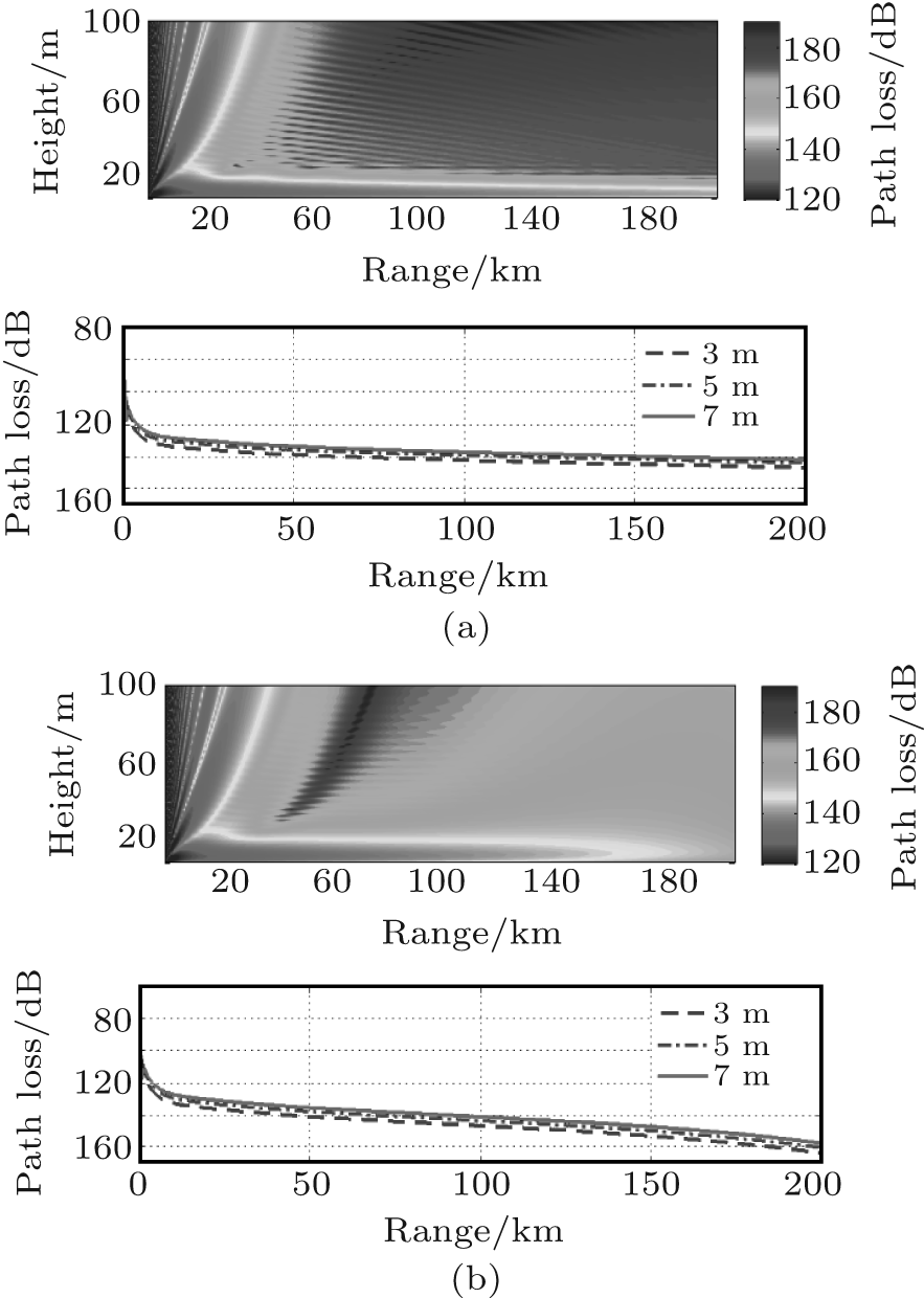 | Fig. 8. Electromagnetic wave propagations in inhomogeneous evaporation duct for EDH = 15 m– 20 m (a), and 15 m– 10 m (b). |
 | Fig. 9. (a) Path losses at 3 m (a) and 200 km (b) in homogeneous and inhomogeneous evaporation ducts. |
Figure 9(b) shows the path loss at 200 km in both a homogeneous and an inhomogeneous evaporation duct. It is shown that when the height is less than 5 m, the path loss in the first case (EDH: 15 m– 20 m) is lowest, about 1-dB lower than that in a homogeneous case. However, the path loss in the second case (EDH: 15 m– 10 m) is highest, about 10-dB higher than that in a homogeneous case. When the height is higher than 20 m, the path loss in the second case is lowest, about 10 dB– 20 dB lower than the first case and the homogeneous case. This is caused by the electromagnetic wave leaking from the evaporation duct in the second case.
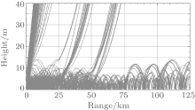
The effect of the horizontal inhomogeneous evaporation duct on the electromagnetic wave propagation can also be illustrated by ray theory. Figure 10 shows the simulation results obtained by using ray theory. The propagation path is 125-km long and the EDH changes every 25 km (14 m→ 10 m→ 7 m→ 10 m→ 14 m). It is shown in Fig. 10 that several rays leak from the evaporation duct as the EDH decreases from 14 m to 7 m. This will cause the path loss to decrease in the evaporation duct. On the other hand, as the EDH increases from 7 m to 14 m, the rays keep propagating in the evaporation duct and the path loss changes slightly.
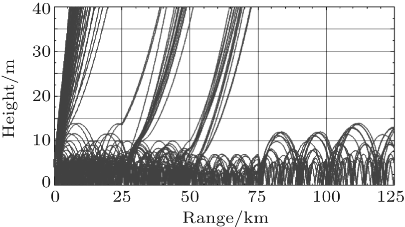 | Fig. 10. Effects of horizontally inhomogeneous evaporation duct on electromagnetic wave propagation (ray theory). |
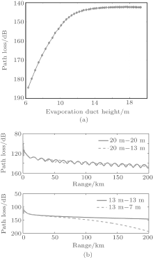
The EDH at the transmitting location is 15 m and the EDH at the receiving location changes from 6 m to 19 m. Figure 11(a) shows the path loss at 3 m with different EDHs at the receiving location. It is shown that when the EDH at the receiving location is lower than that at transmitting location, the path loss is higher than that in a homogeneous condition. When the EDH at the receiving location becomes lower than 10 m, the path loss increases very quickly. For example, when the EDH is 7 m at the receiving location, the path loss is about 175 dB, 30-dB higher than that in the homogeneous case. When the EDH at the receiving location is higher than that at the transmitting location, the path loss is slightly lower than that in the homogeneous case, about 1 dB– 2 dB. Thus, the second case with EDH decreasing has a larger influence on electromagnetic wave propagation.
The horizontal inhomogeneity of an evaporation duct has different influences on electromagnetic wave propagation with different EDHs. Figure 11(b) shows the path losses at 3 m under different evaporation ducts. The transmitting information is the same as that shown in Table 1. When the EDH is low, for example 13 m, the horizontal inhomogeneity of the evaporation duct causes a reduction of 47.5 dB at 200 km compared with the homogeneous case. When the EDH is 20 m, the difference is only about 2 dB at 200 km. Thus, the horizontal inhomogeneity of an evaporation duct has a larger influence on electromagnetic wave propagation when the EDH is low.
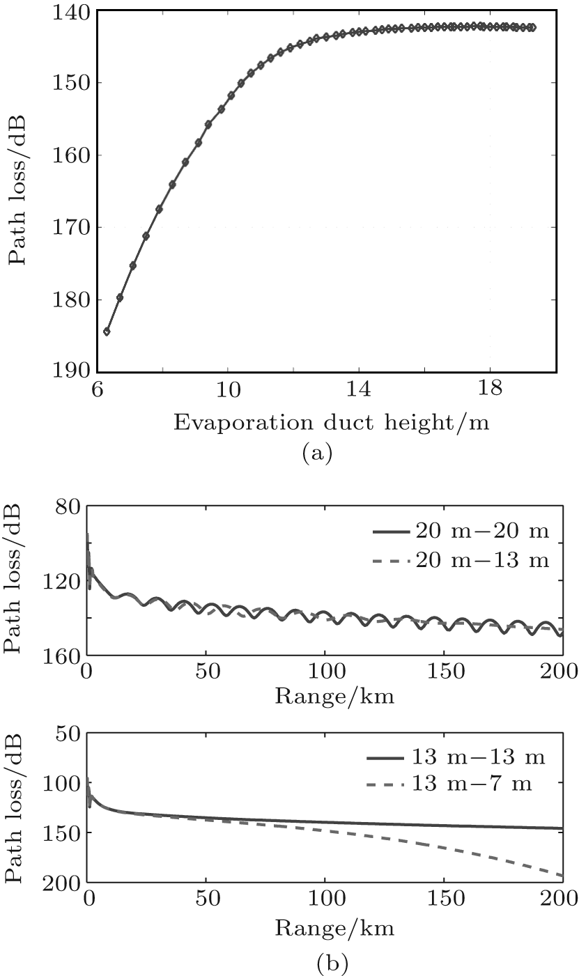 | Fig. 11. (a) Path loss at 3 m versus EDH at receiving location and (b) the path losses at 3 m under different evaporation duct environments. |
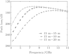
The horizontal inhomogeneity of evaporation duct also has different influences on electromagnetic wave propagations at different frequencies. The frequency changes from 3 GHz to 15 GHz. The environment information and the other transmitting information are the same as those shown in Table 1. Figure 12 shows the path losses at 3 m and 200 km at different frequencies. It is shown that the horizontal inhomogeneity of the evaporation duct exerts a larger influence on the low frequency electromagnetic wave. For example, when the frequency is higher than 13 GHz, both of the two cases only cause a small influence (less than 5 dB) and the influence continues to reduce as the frequency increases. While when the frequency is 5 GHz, the first case (EDH: 15 m– 20 m) causes an increase of 32 dB compared with the homogeneous case. The second case (EDH: 15 m– 10 m) causes a reduction of 39 dB compared with the homogeneous case. This conclusion is consistent with the low frequency cut-off characteristics of the evaporation duct. The following equation determines the longest wavelength trapped in the evaporation duct:

where m(z) is the modified index of the atmosphere at the height of z, and H is the EDH. The electromagnetic wave with wavelength less than λ max (low frequency) can propagate in the evaporation duct.
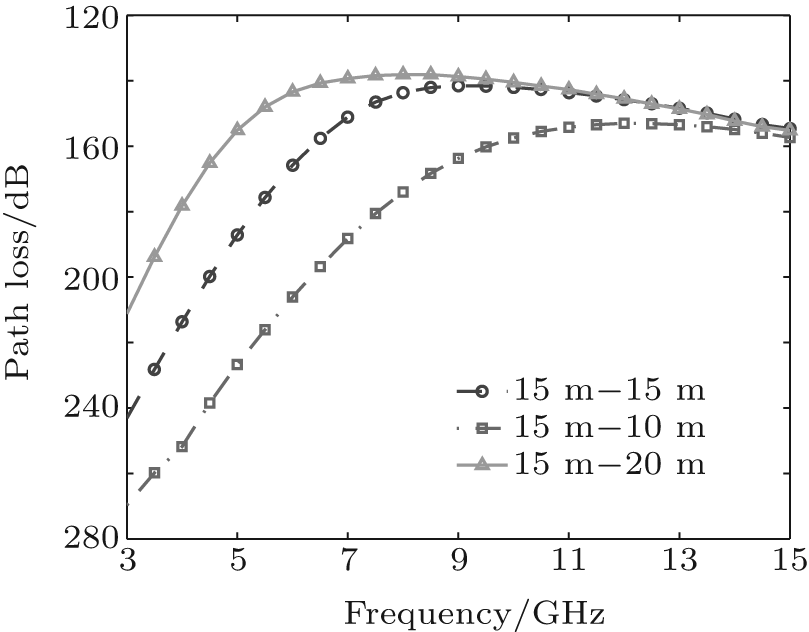 | Fig. 12. Path losses at 3 m and 200 km for electromagnetic wave propagation at different frequencies. |
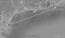
An evaporation duct experiment was conducted in the northern part of the South China Sea in December 2013. The data collected in this experiment was used to verify the conclusion obtained in Section 3. The transmitter was at Donghai Island in Zhanjiang City, Guangdong Province, China. The receiver was at the Hailing Island in Yangjiang City, Guangdong Province, China. The experiment location was shown in Fig. 13 and the propagation path was 149 km.
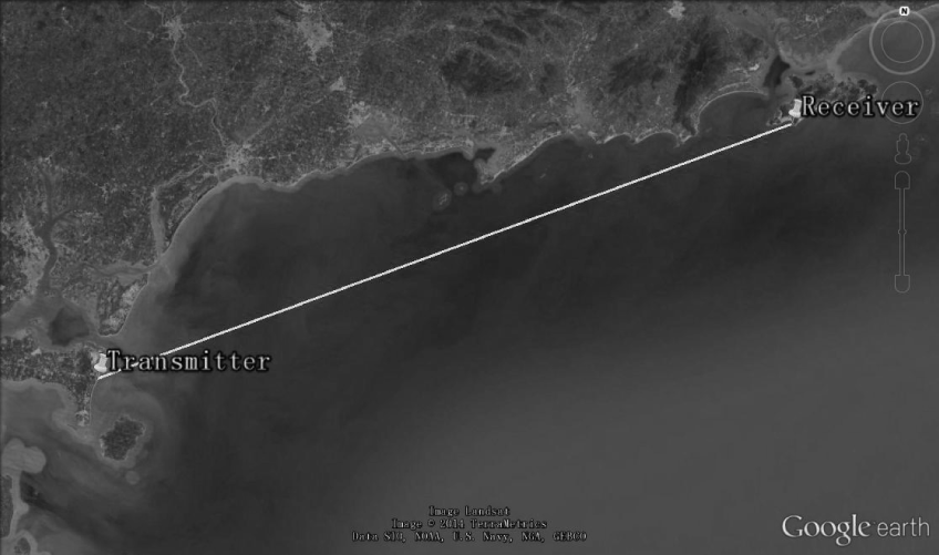 | Fig. 13. Propagation path in the evaporation duct experiment. |
On 30 December 2013, the experiment started at about 8:00 a.m. and ended at 17:00 p.m. (UTC+ 8). The electromagnetic wave was transmitted from the Dong Hai Island and the signal was received at the Hailing Island after propagating about 149 km. The signal frequency was 8 GHz and the received signal level was recorded every second by the computer. The experimental configuration is shown in Table 2.
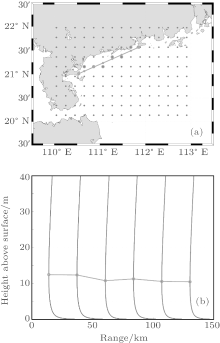
NCEP CFSR data were used to calculate the range-dependent modified refractivity profile along the propagation path. The NCEP CFSR was designed and executed as a global, high resolution, coupled atmosphere– ocean– land surface– sea ice system to provide the best estimate of the states of these coupled domains over this period.[21] One-hour reanalysis data from 1979 to the present day are available, and global atmospheric fields are provided for a variety of atmospheric factors. The spatial coverage has 1152× 576 grid points from 0° E to 359.687° E and 89.761° N to 89.761° S which provides the data with a high horizontal resolution (0.313° × 0.312° ) (Fig. 14(a)). The atmospheric factors shown in Table 3 are extracted from the NCEP CFSR data and input into the NPS model to calculate the modified refractivity (Fig. 14(b)) profile along the propagation path. The grid points which are the closest to the propagation path are used.
| Table 2. Experimental configuration on December 30th, 2013. |
| Table 3. Primary factors and calculated factors from NCEP CFSR. |
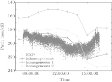
Figure 15 shows a comparison between the experimental results and numerical simulation results. The points are the path loss measured in the experiment. The line with triangles is the path loss calculated by the APM model using range-dependent modified refractivity profiles. The line with rhombus (homogeneous case 1) is the model result only using the modified refractivity profile near the transmitter. The line with circle (homogeneous case 2) describes the path loss calculated by the model using the modified refractivity profile near the receiver. It is shown that the model result with considering the inhomogeneous evaporation duct has less error in comparison with the experimental result. Figure 14(b) shows the range-dependent profile at 13:00 (UTC+ 8) 30 December. The EDH near the transmitter is about 13 m, 3-m higher than the EDH near the receiver. As is discussed in Section 3, when the EDH reduces along the propagation path, the path loss in the inhomogeneous case is lower than that in the homogeneous case. The result shows that the path loss in the homogeneous case is 30-dB higher than the experimental result. However, there is a difference of only less than 10 dB in path loss between the calculated and experimental result if the inhomogeneity of the propagation path is taken into account in the calculations. Therefore, the effect of horizontal inhomogeneity of an evaporation duct on electromagnetic wave propagation is significant and should be considered when modeling the electromagnetic wave propagation near the sea surface.
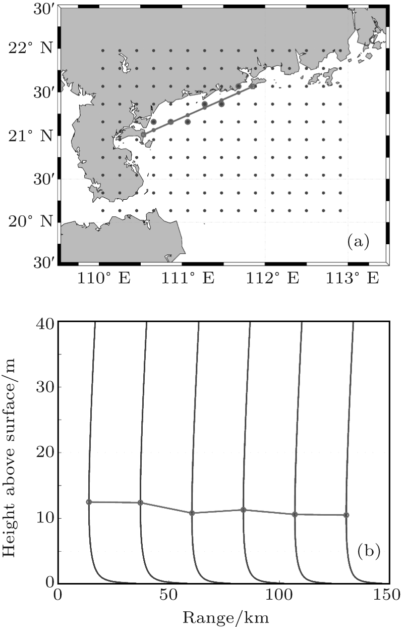 | Fig. 14. (a) Selected grid points of NCEP CFSR on the propagation path, and (b) the range-dependent modified refractivity profile at 13:00 (UTC+ 8) December 30th, 2013. |
It is shown in Fig. 16 that the path loss keeps at about 200 dB from 13:00 p.m. to 15:00 p.m., but the simulation results reduces about 30 dB during these periods. There is an obvious discrepancy between the model results and the experimental results. The APM model is used in the AREPS, which is widely used for the assessment of electromagnetic systems. It is accurate and has also been validated in various environments. The NCEP CFSR reanalysis data are an effective way to obtain range-dependent atmosphere factors along the propagation path. However, the data are the output of data assimilation system and have errors in the areas which lack in-situ observations. The errors of the atmosphere factors are the probable causes of the discrepancy.
 | Fig. 15. Experimental result and the numerical simulation result. |
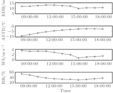
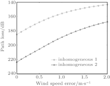
Figure 16 shows the conditions of EDH and atmosphere factors during the experiment (transmitter location). It is shown that the EDH changes from 13 m to about 10 m in a time interval from 13:00 p.m. to 15:00 p.m., which leads to the reduced path loss. The atmosphere is in an unstable condition (ASTD < 0° C) and the relative humidity is in a range from about 30% to 40% . The wind speed decreases from 3 m/s to 1 m/s. The low relative humidity is beneficial to the form of the evaporation duct, so the reducing wind speed leads to a low EDH at 15:00 p.m. Figure 17 shows the influence of the wind speed error on path loss (model results) under the condition of experimental atmosphere. It is shown that if the wind speed increases about 1 m, then the path loss will reduce about 30 dB (in the inhomogeneous cases 1 and 2). The model result is sensitive to the wind speed error and the wind speed error is the probable cause of the discrepancy.
 | Fig. 16. Conditions of EDH and atmosphere factors during experiment. |
 | Fig. 17. Influences of wind speed error on path loss (model results). |
The effects of horizontal inhomogeneity of evaporation duct on electromagnetic wave propagation are studied, both in numerical simulation and experimental observation, in this paper. The features of the horizontal inhomogeneity of the evaporation duct are discussed. The APM propagation model is used to analyze the electromagnetic wave propagation both in a homogeneous and an inhomogeneous evaporation duct. The experimental data collected in the South China Sea in December 2013 are used to verify the conclusion. It is shown that the horizontal inhomogeneity of an evaporation duct has a significant effect on electromagnetic wave propagation near the sea surface. The following conclusions are obtained in this paper.
(i) When the EDH at receiver is lower than the transmitter (i.e., propagation in a wedge), the horizontal inhomogeneity of the evaporation duct causes a significant influence on the electromagnetic wave propagation near the sea surface. The path loss is much higher in this case than in the homogeneous case. While in the opposite case (i.e., propagation in a horn), the influence of the inhomogeneous evaporation duct is slight.
(ii) The horizontal inhomogeneity of the evaporation duct has different influences on electromagnetic wave propagation at different frequencies. In general, the electromagnetic wave propagation at low frequency is affected more seriously by horizontal inhomogeneity of evaporation duct.
(iii) The effect of horizontal inhomogeneity of evaporation duct on electromagnetic wave propagation is serious when the EDH is low on the propagation path.
(iv) The model result considering the horizontal inhomogeneity of an evaporation duct has less error than the experimental result.
The authors express their appreciations to all the participants in evaporation duct experiments conducted in 2013.
| 1 |
|
| 2 |
|
| 3 |
|
| 4 |
|
| 5 |
|
| 6 |
|
| 7 |
|
| 8 |
|
| 9 |
|
| 10 |
|
| 11 |
|
| 12 |
|
| 13 |
|
| 14 |
|
| 15 |
|
| 16 |
|
| 17 |
|
| 18 |
|
| 19 |
|
| 20 |
|
| 21 |
|
| 22 |
|
| 23 |
|
| 24 |
|
| 25 |
|