Theoretical study of amplified spontaneous emission intensity and bandwidth reduction in polymer
Hariri A†, Sarikhani S.
Laser and Optics Research School, North Kargar Avenue, P. O. Box 11365-8486, Tehran, Iran

Corresponding author. E-mail: akbar_hariri@yahoo.com

Abstract

Amplified spontaneous emission (ASE), including intensity and bandwidth, in a typical example of BuEH-PPV is calculated. For this purpose, the intensity rate equation is used to explain the reported experimental measurements of a BuEH-PPV sample pumped at different pump intensities from Ip = 0.61 MW/cm2 to 5.2 MW/cm2. Both homogeneously and inhomogeneously broadened transition lines along with a model based on the geometrically dependent gain coefficient (GDGC) are examined and it is confirmed that for the reported measurements the homogeneously broadened line is responsible for the light–matter interaction. The calculation explains the frequency spectrum of the ASE output intensity extracted from the sample at different pump intensities, unsaturated and saturated gain coefficients, and ASE bandwidth reduction along the propagation direction. Both analytical and numerical calculations for verifying the GDGC model are presented in this paper. Although the introduced model has shown its potential for explaining the ASE behavior in a specific sample it can be universally used for the ASE study in different active media.

Keyword: 32.50.+d; 32.70.Jz; 32.80.–t; amplified spontaneous emission; bandwidth reduction; polymers; gain coefficient
1. Introduction

Amplified spontaneous emission (ASE) is an interesting phenomenon that has been studied both experimentally and theoretically for many years. From the theoretical point of view we may refer to a number of published papers in this subject, including the earliest papers published by Peters and Allen, [1, 2] Casperson and Yariv, [3] Casperson, [4] and Pert.[5] In recent years, on the other hand, with the emerging need of laser materials for their vast applications in laser technology, conjugated polymer films, BuEH-PPV, [6] MEH-PPV, [79] cyano substituted oligo (CN-DPDSB) single crystal, [10] InAs quantum dots, [11] etc., were studied extensively, where due to their importance, the subject has also been reviewed.[12, 13] The most important interest in these studies is to use ASE as a source of coherent radiation. Experimentally, samples under the study are usually excited by pump lasers with an input laser intensity Ip. The results of the measurements are often introduced by plots of ASE intensity, IASE, and bandwidth, Δ λ ASE, versus sample excitation length, lAMP.

For analyzing the experimental measurements, and particularly to determine the ASE gain coefficient, the experimental data points are commonly fitted to an equation given by,

where g0(λ ) is the small signal gain and A is a constant. By using the intensity rate equation and considering the fact that small-signal gain is z-independent, upon assuming that ASE initiates at one end of the sample; that is, using a boundary condition that the ASE intensity is equal to zero at z = 0, equation (1) can be readily obtained.[14]

On the other hand, a particularly interesting feature of the ASE character is that the ASE spectral line narrows while light propagates along the z direction. The earliest study of explaining the spectral narrowing phenomenon was introduced by Yariv and Leite[15] and more elaborate work appearing in Ref. [3], where some approximations were adopted, showed that at large distances the ASE bandwidth reduction, Δ ν ASEν 0, for homogeneously (H) and Doppler (D) broadened line shapes with the ASE bandwidths of Δ ν ASE, H and Δ ν ASE, D are given, respectively, by

where Δ ν 0 and are spontaneous emission bandwidths for H- and D-broadened lines respectively; lAMP is the medium excitation length; and are gain coefficients for H- and D-broadened lines at the zero normalized frequency offset given by x = 2(ν ν 0)/Δ ν 0 and , respectively. Furthermore, in many experimental observations, including in an N2-laser with an excitation length of lAMP = 200 cm, [16] or in a KrF excimer laser of lAMP = 84 cm, [17] it was reported that the ASE intensities start at some values of length threshold zth close to 40 cm and 24 cm, respectively. Also, in our study on gain measurements, upon using an oscillator– amplifier (OSC-AMP) N2-laser system, when the AMPs of different electrode lengths of 2.2 cm to 31 cm were used, we found that for lAMP = 2.2 cm the ASE in the AMP section was eliminated completely.[18] Nevertheless, the light from the OSC section was amplified when it passed through the AMP section. Thus, it should be cited that one particular feature of ASE is its initiation at some threshold length, where it has been observed in all the ASE intensity measurements.

From the theoretical point of view for the behavioral study of the gain coefficient in an OSC– AMP N2-laser system with an amplifier of different excitation lengths, using a mathematical model for N2-lasers as introduced initially by Fitzsimmons et al., [19] we calculated gain coefficients for the AMP section of the laser system for different electrode lengths at instants when the values of gain coefficient, g0(t), were maximal. In this study, we let the cavity lifetime, τ ph, for a traveling wave be some fraction, κ , of lAMP/c, where consequently κ was found to be related to the power loss. c is the light velocity in the medium. With this approach the power loss γ L was introduced into the photon density rate equation. The numerical calculation then showed that γ L is z-dependent and reduces as . By introducing the power loss in the rate equation we were able to numerically calculate gain coefficients for all ranges of the AMP excitation lengths. We also made an analytical approach with considering that at the lasing threshold we can write g0(z)z = γ L (z), where g0(z) is the z-dependent small signal gain. With this realization, we managed to find an analytical expression for the gain coefficient for N2-lasers operating under optimum gas pressures at a constant input voltage, [20, 21] which is expressed below

Here, is the small signal gain at the central band frequency ν 0, and z is the medium excitation length. m′ , , and b are constants, so-called “ gain parameters” , and can be determined by a direct gain measurement for a given medium with different excitation lengths using, for example, an OSC– AMP laser system. As b was found to be generally a small quantity, then, with a good approximation we can let b = 0 and keep the loss factor equal to which is a constant and independent of the z direction. The z-dependent gain profile given by Eq. (3) appears to predict a high value for the gain coefficient for small z; while for large z, it reveals a low value for the gain coefficient. This is a fact that has appeared in all the reported gain measurements using different gain media of different geometrical dimensions. The value of m′ in Eq. (3) depends on the laser system, type of laser material, excitation mechanism, saturation effect, etc., and it was initially introduced to remove the inequality of ∂ nph/∂ t > 0 for a self-sustained oscillation for the photon density nph. Although equation (3) was obtained for an N2-laser under its optimized operational gas pressure, but it was verified that it is capable to predict gain coefficients in self-terminating gas lasers such as excimer lasers, , N2, F2, CVL reported from different laboratories.[21]

About the study of the ASE phenomenon, on the other hand, for explaining the ASE output energy in a KrF laser, i.e., ε ASE versus lAMP, gain coefficients for different segmented excitation lengths were calculated and it is observed that the calculated ASE gain coefficients also obey an equation similar to Eq. (3). With the available experimental measurements, as specific examples, equation (3) was used to predict the ASE output behavior in KrF[2225] and N2[26, 27] lasers, and we found that the corresponding ASE gain profiles, denoted by and , obey Eq. (3) with slightly different gain parameters, compared with those obtained by direct gain measurements. In fact, the corresponding turned out to be slightly lower than the gain profile drawn from the collected KrF or N2 lasers gain coefficients versus the excitation length reported from different laboratories. Thus, with a complete study of gas lasers it was verified that the gain coefficient depends strongly on the geometry of the laser system when the system is in its optimum operational conditions.

In general, for applying the model of geometrically dependent gain coefficient (GDGC) with a plot of measured ASE output energy or intensity versus excitation length for a given sample, we can obtain gain parameters for the excited sample, and consequently the ASE gain profile, , will be determined. With this realization, the gain coefficient for the sample for the length of z = lAMP can be obtained readily by using Eq. (3).

In the present work we use Eq. (3) along with the intensity rate equation to explain the ASE behaviors in organic solid materials theoretically. These materials are prepared in small-sized dimensions. For the study, we include the threshold length zth in our analysis. Although the values of zth are very small in these materials due to their small dimensions, but it is important to take them into consideration in the calculation to obtain a correct prediction for the ASE behavior. In fact, in the reported measurements of organic materials, the presence of the threshold lengths in the experimental measurements is visualized clearly. For verifying the geometrical model of the gain coefficient in small-sized materials, we use the reported measurements of the intensity and ASE bandwidth reduction along the excitation length. For the study of the spectral behavior, by the use of an analytical approach, we find that the output intensity spectrum for ν ν 0, or x2 ≪ 1, for high pump intensity, Ip, has a Gaussian distribution when initially a homogeneously (H) broadened line shape is used for the calculation. We will show that this condition is also satisfied for long enough excitation lengths when the narrowing of the ASE bandwidth occurs. For x2 ≫ 1, or in the earlier stage of the ASE propagation, the intensity behavior has a Lorentzian frequency distribution. On the other hand, our calculations show that when initially an inhomogeneously or Doppler (D) broadened transition is used, the intensity profiles for both x2 ≪ 1 and x2 ≫ 1 turn out to be Gaussian functions. To observe the details of the bandwidth narrowing, the numerical calculations for the ASE intensities for homogeneously and inhomogeneously broadened line shapes are also carried out. For the analysis that is made for the BuEH-PPV sample, it is determined that a homogeneously broadened transition is responsible for the broadening mechanism. The results indicate that the approach gives excellent consistency with the measurements for the whole range of the sample excitation lengths and for different pumping conditions. In particular, we realize that the saturation effect has an important influence on the analysis. When the saturation effect is introduced in the intensity rate equation, the results of the calculated intensity for H-broadened lines show that when light propagates along the z direction, the intensity profile in a logarithmic scale versus excitation length z, has a sharp and subsequently a smooth bending curvature. Consequently a saturation length, zsat, which refers to a length at which the ASE intensity is equal to the saturation intensity, is defined. In contrast to Eq. (1) that cannot explain the experimental data in the whole range of measurements, fittings of the experimental data, by applying the present model, are found to be well performed. In addition to the unsaturated gain coefficient, , we are also able to predict the saturated gain coefficient, . In general, the present approach can be considered as a reliable method of analyzing the relevant experimental measurements, and thereby confirms the validity of the proposed GDGC model to be applicable for samples of different types and dimensions. As the model simplifies the analysis of the ASE measurements, it can be used as a reliable tool for investigating the details of mechanisms involved in the interaction between light and matter. The model provides gain parameters, where with good accuracy, these parameters may be used for studying the saturation effects, type of broadening, ASE bandwidth, etc.

2. Theoretical approach

The analytical approach to explain the ASE behavior, using a four level system for a homogeneously broadened transition, has led to an analytical expression for the ASE output energy or intensity, and has been introduced in Refs. [22] and [23]. Thus, the details of this part of the calculation are not given here, except some relevant parts for better understanding of the proposed method. In this work, in addition to extending the analytical considerations for different conditions that appear in experiments, specific attention will be paid to the numerical calculations, and the corresponding results are introduced by graphs and the deduced relevant parameters are tabulated. Comparisons between numerical and analytical results for explaining experimental measurements will be also given to elucidate the ASE behavior in a small-sized sample completely.

2.1. Homogeneously broadened transition

For calculating the ASE intensity Iν and bandwidth Δ ν ASE for the steady-state solution, we start with the intensity rate equation when the saturation effect is not included in the rate equation, i.e.,

Here, τ sp is the medium upper state radiative lifetime. For a four level system the upper-state population N2(z) is related to the gain coefficient by , where is the small signal gain at frequency ν ; is the stimulated emission cross section at frequency ν , where for a homogeneously (H) broadened line shape it is given by . In this equation x = 2(ν ν 0)/Δ ν 0 is the normalized frequency offset, and is the stimulated emission cross section at the transition frequency ν 0. Thus, for in this case, we can write . To reach a closed form relation for Iν (z), the factor γ (z) appearing in Eq. (4), i.e., γ (z) = Ω (z)/4π has to be taken to be a constant, otherwise it is impossible to obtain an analytical formulation for Iν (z).[14]Ω (z) is the solid angle subtended by the exit face of the sample as seen from a point in the center of a plain surface located at the z position of the medium.[14]γ (z) describes the characteristics of the ASE propagating along the z direction. As mentioned in Ref. [23], evaluation of γ (z) at zth gives a reasonably good approximation compared with the case when the explicit expression for γ (z) is used in the numerical calculation. In fact for the case of using γ (zth), the analytical solution turns out to be very close to the numerical solution. However, to obtain a more accurate result, it is required to evaluate the value for γ (z) by considering the fact that the numerical calculation for Iν (z) should be overlapped with that of the analytical solution. The corresponding symbol in this case is shown by γ num in the text.

The second term on the right-hand side in Eq. (4) is , and the solution of Eq. (4) for Iν (z) is given by the following expression:[22, 23]

where is defined by the following integral

It should be emphasized that at z = zth, the ASE intensity is equal to zero and this constitutes the boundary condition for solving the intensity rate equation.

For the saturation intensity at frequency ν , we can use

Here, ϕ is the fluorescence quantum yield, given by ϕ = τ u/τ sp, where τ u is the medium upper state lifetime. By introducing and defining , equation (5) is simplified into

This is the general solution for the ASE intensity at the transition frequency ν . For the z-independent value of from Eq. (6) we obtain . By considering zzth = lAMP, then the term in Eq. (8) will be evaluated to be equal to . On the other hand, in the steady state condition, the upper state population is obtained using Rp = N2/τ u, where Rp is the pumping rate and is given by Rp = α absIp/p.[14] The α abs is the absorption coefficient of the medium at the pump frequency ν p, and Ip is the pump intensity.[14] By using Eq. (7) and , equation (8) with this assumption gives

Here, we may define A(ν ) = γ (zth) α absϕ ν /ν p for any transition frequency ν . From Eq. (8a) we finally obtain

It is seen that equation (8b) is the same as Eq. (1) when we let IASE(lAMP) ≡ Iν (lAMP). It is also a simplified form of Eq. (8) on the assumption that the gain coefficient is z-independent. Here, ν = c/λ is also applied.

For applying Eq. (8), two cases for the analytical solution for an H-broadened system may be considered.

Case a For ν ν 0 so as to obtain the x2 ≪ 1 condition, we can further use Eq. (8) and apply this equation to the H-broadened line transition. In this case, we use symbols of and for and terms as they appear in Eq. (8), respectively. Consequently, we have

where is given by

and we also define , where is given by Eq. (3). It deserves to be mentioned that , according to Eq. (3), is introduced by three parameters that are different for H- and D- broadened lines. However, for simplicity we drop H and D notations for , and , by keeping in mind that gain parameters are different for H- and D- broadenings. We also let . If we substitute according to Eq. (9) into Eq. (8), and knowing that the term is also a function of line spectrum, we obtain

By expanding the second term inside the brackets and upon neglecting the terms with x2, x4, … factors, we obtain finally,

In the plot of Iν (z) versus x for a given z, if the Iν measurements appear to follow Eq. (11a), then one can expect to obtain a Gaussian frequency distribution. By defining the saturation length, zsat, the numerical calculation, in fact, shows that the x2 ≪ 1 condition corresponds to a large z; that is, the condition when zzsat is satisfied. This refers to the present study of the H-broadening when the total medium is pumped optically with a high pump intensity Ip, where zzsat is satisfied.

The presence of the term in Eq. (11a) guarantees the boundary condition of Iν (z = zth) = 0. Equation (11a) shows clearly that according to the model of the geometrically dependent gain coefficient, the ASE intensity for ν ν 0 has a Gaussian distribution with a full width at half maximum (FWHM) given by

By applying the x = 2(ν ν 0)/Δ ν 0 to getting Δ xASE, H = 2Δ ν ASE, Hν 0, we obtain the ASE bandwidth reduction,

where Δ ν 0 is the spontaneous emission bandwidth for the H-broadened line.

By using the gain formulation as given by Eq. (3), and evaluating the integral, we obtain

and

from which we finally reach the following analytical expression for the ASE bandwidth reduction along the z direction for the case when zzsat is satisfied:

It is interesting to see that by ignoring the last two terms in Eq. (14a), and by letting , we obtain exactly Eq. (2) for the H-broadened line introduced initially in Ref. [3].

The stimulated emission cross section for the homogeneously broadened line shape at ν = ν 0 is given by , where 𝔤 ν 0, H is the value of the line shape at the band center ν 0, and given by 2/π Δ ν 0. Thus, we can express given by Eq. (7) in terms of Δ λ 0 (the spontaneous emission spectral width), as

where can be determined experimentally.

Case b For the x2 ≫ 1 condition, where it also corresponds to the zzsat condition, say, at the earliest stage of the ASE propagation, we may again use Eq. (8). If we let , the term which appears in this equation can be expanded to give

By keeping the first three terms in Eq. (17), and under the condition which is imposed on Eq. (8), then equation (8) is written as

where again for the H-broadening has been used. Equation (18) shows clearly that for x2 ≫ 1, the ASE intensity has a Lorentzian distribution added to a constant value of is given by

For x → ∞ , we obtain a constant value for Iν (z), which is ν 0-dependent. Here, we can define the expression . In this case equation (19) can be written as

Equation (19a) shows that Iν (z) has a Lorentzian frequency distribution at any distance z if the term, which is a constant, is removed from the equation. Then, if we define , we can calculate the FWHM value in this condition,

That is, under the condition of x2 ≫ 1, the ASE bandwidth is the same as the spontaneous emission bandwidth.

For a very large x, the FWHM can be obtained from Eq. (19a) analytically when the term is also considered in the FWHM calculation, i.e.,

where the term in Eq. (20) means . Furthermore, by keeping four terms, we reach the following second order equation:

where ξ = 1/(1 + x2) is defined. For the positive solution of Eq. (21), we obtain

and Δ ν ASE, Hν 0 is obtained, accordingly,

Thus, for the H-broadened transition, we observe that without including the saturation effect, equation (5) or (8) can explain the ASE intensity in general, and at two limits of x2 ≪ 1 and x2 ≫ 1, the analytical solutions as given by Eqs. (11a) and (19a) turn out to be a Gaussian and a Lorentzian frequency distribution, respectively. This prediction will be verified by the experimental measurements and also by the corresponding numerical calculations.

2.2. Inhomogeneously (Doppler) broadened transition

We may apply the previous procedure as given in Subsection 2.1, to the Doppler (D) broadened transition. For the stimulated emission cross section, we have , where , and the line width at ν 0 for a D-broadened system is given by , where is the Doppler broadened bandwidth.[14] For therefore, we can write . For the Iν (z) calculation, we again use Eq. (8), and obtain

where for we use . Two cases are also considered here.

Case (i) For ν ν 0 or x2 ≪ 1, we can approximate ex2ln 2 ≈ 1 − x2ln 2, and consequently equation (24) turns out to be

where means . For lAMP ∼ 2 mm in this example, is close to 12, so two exponential factors in the front of the brackets, i.e., can be approximated to . By expanding the second term inside the brackets appearing in Eq. (25) and for x2 ≪ 1 by keeping the first term in this expansion, we have

Equation (26) shows that the ASE intensity has a Gaussian frequency distribution for x2 ≪ 1, which will be shown to correspond to the zzsat condition. The FWHM can be obtained easily from this equation,

By ignoring the last two terms in Eq. (14a) and by letting zzth = lAMP and , we obtain Eq. (2) for the case of D-broadening if equation (27) is used. Here again we observe that Iν (z) for x2 ≪ 1 has a Gaussian frequency distribution.

Case (ii) For x2 ≫ 1, i.e., in the earliest stage of the ASE propagation along the z direction, or when zzsat is satisfied, the first exponential term inside the brackets in Eq. (24) can be expanded to yield

By keeping the first 3 terms in the expansion, we have

Equation (29) shows that the intensity spectrum again has a Gaussian distribution added to a constant value given by . Thus, for the D-broadened line in this case we obtain

which shows that Iν (z) has a Gaussian frequency profile if the term, which is a constant background of the intensity in a measurement, is removed, i.e., by defining . In this case, the ASE bandwidth has the same value as the spontaneous emission bandwidth, i.e.,

The introduced analytical expression appearing in these two subsections along with the numerical calculations that will be given in Section 3, are used to explain the experimental observations appearing in the article by McGehee et al.[6] Generally, we learn from Subsections 2.1 and 2.2 that according to the initial frequency distribution of the line-shape, which is either a Lorentzian or a Gaussian function, the ASE intensity distribution for zzsat (or x2 ≪ 1) has a Gaussian distribution. For zzsat (or x2 ≫ 1), on the other hand, if we start with a homogeneously broadened transition, the IASE has a Lorentzian line-shape and for an inhomogeneously broadened system IASE has a Gaussian frequency distribution. Thus, with the output spectrum measured at the exit face of a pumped sample, and by knowing the numerical value of zsat one can make an accurate evaluation for the initial frequency distribution for the type of the broadening mechanism involved in the interaction.

3. Numerical calculation

We may consider solving the problem numerically, where saturation and frequency dependences of the gain coefficient are taken into account in the intensity rate equation. For this purpose, from Eq. (4) is replaced by . The notation μ is used for unifying the three equations used in this study. μ takes values of μ = 0, 1/2, 1, where μ = 0 refers to the case where the saturation effect is not considered for the calculation. μ = 1/2, 1 refer to the saturated with the inhomogeneously broadened transitions, and the saturated with the homogeneously broadened transitions, respectively. Thus, the intensity rate equation in a single equation can be written as

Equation (31) is a general equation for the intensity rate equation and can be used according to our needs. For example, for the investigation of the output spectrum when the effect of saturation is not included in the intensity rate equation, we may let μ = 0. In this case for the H-broadening from Eq. (31) we have,

To obtain Eq. (32) we have also used , and . For the case of Doppler broadening, the ex2ln 2 term is replaced by the 1/(1 + x2) term appearing in Eq. (32), and for we have used , where is given by Eq. (16). Thus, for the bandwidth calculation at any distance zi for a homogeneously broadened line shape, for example, equation (32) must be solved numerically using x as a parameter and let it vary in a wide range of the normalized frequency offset to obtain Izi(x). The FWHM of Izi(x) gives Δ ν ASE, H at the specific distance zi. When the calculation is carried out for all the values of given zi, we will obtain the Δ ν ASE, H-profile, i.e., Δ λ ASE, H with respect to z. For considering the effect of saturation, μ = 1, or 1/2 is used in Eq. (31) for homogeneously or Doppler broadened line shapes, respectively. For the -profile, again, we use its analytical expressions, given by Eq. (3) as mentioned earlier. For μ = 1/2, a Voigt integral should be used, where inside the square root of Eq. (31) should be replaced by .[26]

For the calculation of the ASE intensity at the resonance transition of ν = ν 0, we let x = 0, and consequently Iν 0(z) is calculated. When the effect of saturation is not considered, μ in the intensity rate equation is equal to zero, whereas by including the saturation effect, μ is equal to 1 or 1/2. For the numerical calculation, it is necessary to use the z-dependency of γ (z). As we deal with a small-sized sample having a width of dAMP and a thickness s, we use γ (z) = sdAMP/4 π z2 throughout the calculation. Here, we examine the H- and D-broadenings, both, and consequently we solve the equations with μ = 0, μ = 1, and μ = 1/2 conditions. As both solutions for the cases of using (μ = 0, 1) or (μ = 0, 1/2) explain one set of experimental data points, the corresponding solutions for each case must be overlapped with different gain-parameters. The intensity profiles corresponding to the numerical solutions start at a threshold length zth, and increase along the z direction. The results corresponding to the numerical and analytical approaches are given in Section 4, and the corresponding parameters for the H-broadened system appearing in the relevant calculated graphs are also summarized in Table 1.

Table 1. Deduced gain parameters and threshold lengths and gain coefficients for lAMP = 0.2 cm.
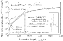
Fig. 1. Plots of the ASE intensity versus excitation length. Sample thicknesses are: s = 150, 200, and 300 nm. The calculations are carried out when μ = 1 is used for H-broadening (C1, H-profiles). The refers to the calculation for μ = 0, with gain parameters obtained from the C1, H-profile with s = 200 nm, and it refers to the unsaturated intensity calculation. The inset shows the chemical structure of the polymer.

Fig. 2. Plots of the ASE calculation with μ = 0 (dashed line), and μ = 1 (solid line), showing the effect of the saturation effect in the intensity rate equation. The C1, H-profile is borrowed from Fig. 1, and compared with the C0-profile. The inset shows the analysis when equation (1) is used for fitting to the linear part of the measurement in a logarithmic scale. Measurements are given in Ref. [6].

4. Results of numerical calculations

To observe the validity of the GDGC model, we use the experimental measurements for planar wave guides of BuEH-PPV reported by McGehee et al.[6] For the calculation, initially, the following parameters are used: λ 0 = 562 nm, s = 200 nm, and dAMP = 350 μ m (s is the thickness and dAMP is the width of the target). n = 1.76 is the sample index of refraction. Δ λ 0 = 47 nm is the measured spontaneous emission bandwidth. In Ref. [6], the experimental measurements of IASE versus excitation length are given with four different pumping intensities of Ip = 0.61, 1.2, 2.2, 4.1 kW/cm2. The measured ASE bandwidths are also given by plots of Δ λ ASE versus excitation length for Ip = 0.61 kW/cm2 and 4.1 kW/cm2. The gain parameters deduced from the IASE versus lAMP measurements should also be able to predict the Δ λ ASE versus lAMP measurements. This is the first criterion for a proper evaluation of the gain parameters. The second requirement is to have the μ = 0 and μ = 1 for H-broadening (or μ = 0 and μ = 1/2 for D-broadening) intensity solutions to be approximately overlapped with different gain parameters. This requirement is due to the fact that in the IASE versus lAMP experiment, we have just one set of measurements and the intensity rate equation should be able to explain the occurrence of the ASE event no matter whether applying the saturation effect in the rate equation or not. The third requirement is to have the solutions to predict just one value for the threshold length zth. In fact, the ASE intensity starts at zth and then grows along the z direction, the saturation will start to affect the ASE intensity gradually. Naturally, the inclusion of the saturation effect in the intensity rate equation should not change the z position of the threshold length. The fourth criterion is to use the measured ASE spectra, introduced by the plots of IASE versus wavelength, and confirm them by using the GDGC model. Finally, the fitting of experimental data to the model must be accomplished perfectly for the whole range of excitation lengths. With these restrictions, the gain parameters can be determined within a relatively small error due to the parameters fitting procedure.

The fluorescence quantum yield of 0.62 is given in Ref. [6], then it must be identified with one of the IASE versus lAMP experimental plots it belongs to. With the upper state lifetime τ u, nonradiative lifetime τ nr, and , we obtain ϕ = 1/(1 + Knrτ sp), which shows that by increasing Knr, the fluorescence quantum yield decreases and consequently we obtain a higher value for the saturation intensity. To see the effect of ϕ in the calculation, we also examine ϕ = 0.2, and find that regardless of small changes that occur in the gain parameters, the calculated results are close to the case when ϕ = 0.62 is used. Thus, ϕ = 0.62 is considered throughout the calculations.

4.1. H-broadening: calculation of Ip = 4.1 kW/cm2 (high pump intensity)

For the input pump intensity of Ip = 4.1 kW/cm2 and ϕ = 0.62, the calculated output intensity at ν = ν 0 is given in Fig. 1. In this calculation is applied. To use the experimental measurements, the scale of intensity is modified according to the calculated value of . Gain parameters, m′ , , and b, are obtained by changing them continuously so as to obtain the best fittings to the intensity and bandwidth experimental observations simultaneously. The C1, H profiles in this figure refer to the μ = 1 solution when H-broadening is used. The saturation lengths, zsat, corresponding to the calculations with s = 150, 200, and 300 nm are slightly different and lie in a range of 0.08 cm– 0.09 cm. This length corresponds to a length at which the ASE intensity is equal to . The total length of the sample is lAMP = 0.2 cm, and it is seen that at this pumping level, the zsat < lAMP condition is satisfied. The , calculated for s = 200 nm, corresponds to the case where μ = 0 is considered, while the gain parameters from the C1, H-profile are used. Thus, the refers to the unsaturated ASE intensity. The corresponding gain parameters are tabulated in Table 1. In Fig. 2, the solution with μ = 0 is shown by the C0-profile. This profile is comparable to the C1, H-profile given in Fig. 1. Both profiles with a negligible error explain the IASE measurement and their threshold lengths are very close to each other as shown in this figure. They are 0.0045 cm (for μ = 1) and 0.0055 cm (for μ = 0). In the inset of this figure we also introduce the plot analyzing the measurement when equation (1) is used. In Fig. 3, based on the gain parameters deduced from solutions of the rate equation, gain coefficients are calculated and they are shown by profiles corresponding to the saturated gain profile with the μ = 1 solution (G1, H-profile), unsaturated condition when the gain parameters from the G1, H-profile are used in the μ = 0 solution , and the saturated condition with the μ = 0 solution (G0-profile). The saturated gain profiles for μ = 0 and μ = 1 solutions (i.e., G0 and G1, H-profiles) are slightly different, showing that the gain parameters, although they are remarkably different in their values, introduce approximately the same saturated gain profiles of the pumped sample. The unsaturated gain profile, as expected, is higher than the saturated gain profile, and for lAMP = 0.2 cm, it is calculated to be 65.8 cm− 1, which is slightly higher than the value of 62 cm− 1 reported in Ref. [6], when equation (1) is used for analysis. The saturated gain coefficients for lAMP = 0.2 cm corresponding to G1, H and G0-profiles are 8.3 cm− 1, and 14.0 cm− 1, respectively. As for large enough z, we expect to obtain the saturated gain coefficient to approach to a small value and also the effect of saturation on the IASE-profile can be observed for the μ = 1 solution, so we consider the saturated gain coefficient corresponding to the μ = 1 intensity solution, i.e., gν 0 = 8.3 cm− 1 for Ip = 4.1 kW/cm2, to be used in the plot of gν 0 versus Ip. It clearly follows from this example that when small-sized samples are pumped at a high light intensity, the GDGC model gives two different values for the saturated and unsaturated gain coefficients, to some extent the unsaturated gain coefficient can also be predicted by Eq. (1). This is due to the measurements under high pump intensities which appear with sharp rises of the IASE versus excitation length in a logarithmic scale. However, equation (1) definitely does not predict the saturated gain coefficient, as it is given in this article. Further difference regarding the potential of the model will be given in Subsection 4.4.

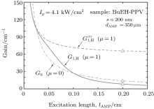
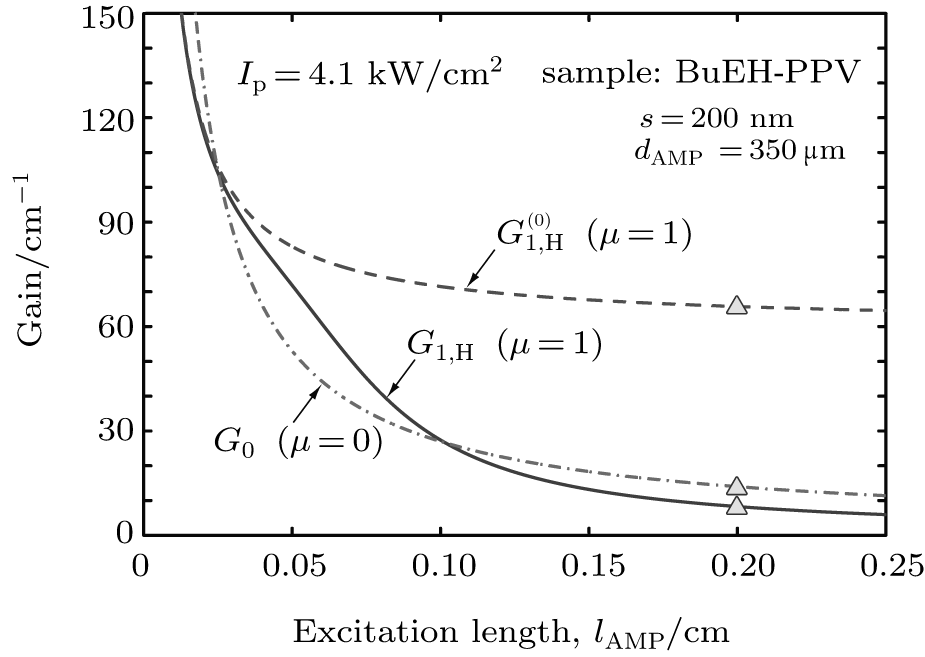
Fig. 3. The saturated G1, H and G0 gain profiles for the μ = 1, and μ = 0 calculations, according to the deduced gain parameters given in Table 1. The corresponds to the unsaturated gain coefficient. For an excitation length of lAMP = 0.2 cm, the saturated gain coefficients corresponding to excluding and including the saturation effect in the rate coefficient are gν 0 = 14.0 cm− 1 and 8.3 cm− 1, respectively. The unsaturated gain coefficient is 65.8 cm− 1. This gain value should be compared with , analyzed by Eq. (1) and is reported in Ref. [6]. The corresponding gain values for lAMP = 0.2 cm are shown by symbols (△ ).

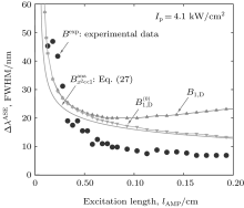
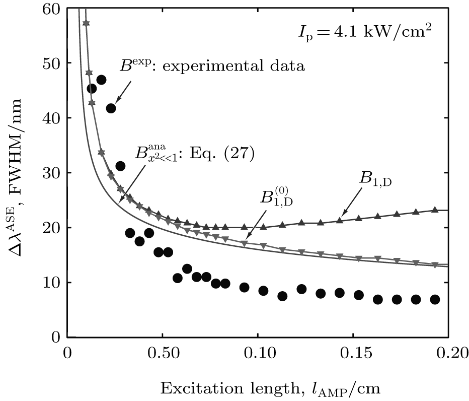
The calculated bandwidths for Ip = 4.1 kW/cm2 are shown in Figs. 4(a) and 4(b). In Fig. 4(a), in addition to the numerical calculations, the experimental measurements of (Δ λ )ASE, shown by the Bexp-profile are also introduced. According to three different views for the previously introduced calculations of the saturated and unsaturated intensity profiles, here three different views for the calculated bandwidths are also given. They are shown by the B0, B1, H, and for the H-broadened transition: B0 refers to the case where μ = 0 is applied; B1, H is given for the case where μ = 1 is used, and finally the represents the solution with μ = 0, but gain parameters are used from the B1, H-profile. These profiles show that the unsaturated bandwidth is very close to the Bexp-profile at large distance. This calculation for the ASE bandwidth shows that the saturation effect causes a bandwidth rebroadening, which is inconsistent with the measurements. In Fig. 4(b) the results of the numerical calculation for the unsaturated condition, shown by , are compared with the analytical calculations for x2 ≫ 1, shown by , and for x2 ≪ 1, shown by . In this figure the Bexp-profile is also shown to observe the degree of consistency between the analytical solution and the measurements. At large z, when the condition of x2 ≪ 1 is satisfied, the bandwidth that is shown by the and given by Eq. (13), becomes close to the experimental measurements, whereas for short distances, i.e., when the condition of x2 ≫ 1 is applied, equation (23) is able to explain the measurements as shown by the . This calculation confirms that a Lorentzian line-shape for zzsat, which corresponds to x2 ≫ 1, can explain the ASE bandwidth behavior. That is, at the earliest stage of the ASE propagation, the bandwidth is explained by a Lorentzian line-shape. This figure also clearly shows that the analytical approaches for two limits of small and large z are consistent with the numerical calculations and also with the experimental measurements.

Fig. 4. (a) Plots of the calculated ASE bandwidth versus the excitation length. The B0-profile corresponds to the μ = 0 solution. The B1, H-profile for μ = 1, and the for μ = 0, but in this case gain parameters from the B1, H-profile are used. Profiles refer to the saturated (B0 and B1, H-profiles) and unsaturated bandwidths. (b) To compare the with the analytical formulations, this profile is introduced, showing the overlapping of the solutions (for x2 ≪ 1 and x2 ≫ 1) with the and the measurements. The refers to Eq. (13). The refers to the calculated bandwidth for using three terms [Eq. (23)] in the expansion appearing in Eq. (17). The values of Bexp in both figures refer to measurements.[6]

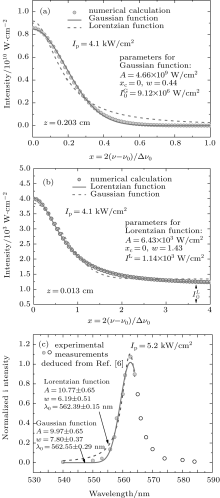
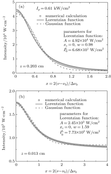
The numerical calculations for the ASE output intensity versus x for large and also short distances (for example z = 0.203 cm and z = 0.013 cm, respectively) are carried out and the results are given in Figs. 5(a) and 5(b), respectively. For identifying the calculated intensity distribution, a Gaussian and a Lorentzian function of the type

and

are fitted to the numerically calculated profiles, and the parameters , , A, xc, and w are determined separately. The large distances (i.e., zzsat) correspond to very small x, where the condition of ν ν 0 is satisfied. In this case, as shown also in the analytical approach, the ASE intensity has a Gaussian distribution. This is indicated in Fig. 5(a), showing that for z = 0.203 cm the intensity favors a Gaussian distribution compared with a Lorentzian line-shape. For z = 0.013 cm which corresponds to a large x, we observe that the ASE intensity favors a Lorentzian line-shape. For x → ∞ also we obtain from Eq. (19) that . This distance is also indicated in Fig. 5(b). The parameters obtained in this case are , xc = 0, w = 1.43, and A = 6.43 × 10³ W/cm2. Thus, is considered as a good parameter to verify that the intensity has a Lorentzian distribution. For the value of zth = 0.0045 cm, we obtain γ (zth) = 0.0028. Also, is equal to 1.73 for z = 0.013 cm. The calculated value of for using γ (zth) is 2.96 × 10³ W/cm2, which gives an error of 160% compared with the fitted value of 1.14 × 10³ W/cm2. Thus, a better value for γ (z) for this evaluation is needed. The numerical calculation for the intensity to obtain an overlap with the analytical calculation gives γ num = 0.0012. This value corresponds to z = 0.0068 cm which is slightly higher than zth, and in this case is equal to 1.27 × 10³ W/cm2. This calculation gives an error of 11% with respect to the fitted value of 1.14 × 10³ W/cm2. The present argument definitely indicates that at large x (or small z), when the ASE propagation is in its earliest stage, the ASE frequency distribution is a Lorentzian function when an H-broadened transition is initially used for the calculation. A clear deviation of the fitted Gaussian function from the exact numerical calculation is clearly shown in Fig. 5(b). Calculations for the intensity profiles are also extended for two different values of z: one is slightly lower and the other is slightly higher than zsat, i.e., z = 0.073 cm and z = 0.093 cm, and we find that both Lorentzian and Gaussian distributions have equal contributions on the transition from a Lorentzian to a Gaussian function at the saturation length (zsat = 0.085 cm). This also indicates that the transition occurs smoothly. We can further refer to the measurement given in Fig. 5(c) for the output intensity spectrum at the exit face of the pumped sample at Ip = 5.2 kW/cm2, and this figure also verifies that the ASE has a Gaussian frequency distribution at the high pump intensity. As the narrowed spectrum has 0– 0 and 0– 1 vibrational peaks, the fitting is accomplished using the leading part of the fluorescence spectrum corresponding to the 0– 0 vibrational peak.

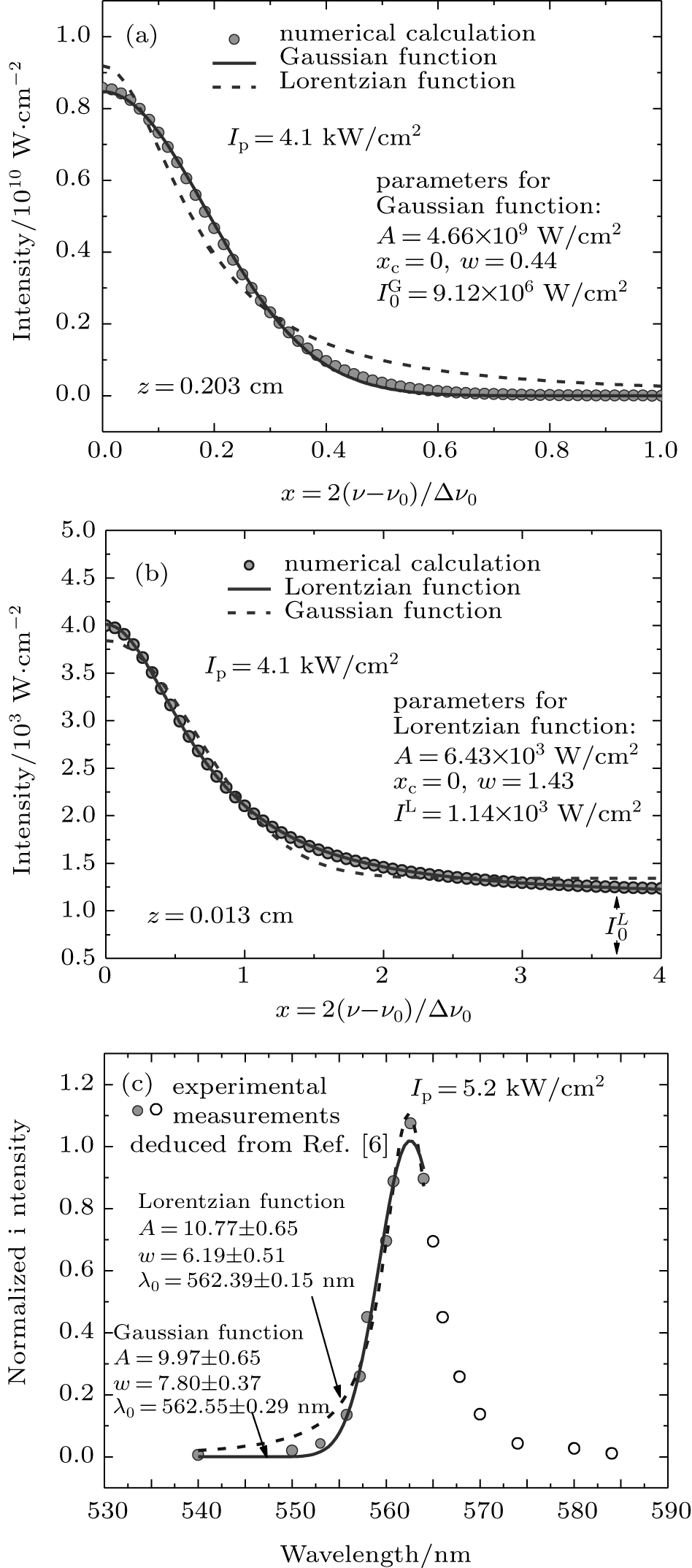
Fig. 5. Plots of the calculated ASE intensity versus normalized frequency offset x = 2(ν ν 0)/Δ ν 0 (a) for z = 0.203 cm, showing that the calculated intensity favors a Gaussian distribution and verifies the x2 ≪ 1 approximation for the intensity; (b) for z = 0.013 cm, showing that the calculated intensity has a Lorentzian distribution and that corresponds to the x2 ≫ 1 approximation. Both panels (a) and (b) correspond to Ip = 4.1 kW/cm2; (c) the plots of normalized ASE intensity versus wavelength for Ip = 5.2 kW/cm2 measurements as given in Ref. [6]. The experimental measurements show that IASE at high pump intensity, when zzsat is satisfied, favors a Gaussian frequency distribution.

4.2. H-broadening: calculation of Ip = 0.61 kW/cm2 (low pump intensity)

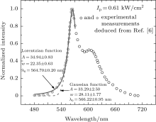
For Ip = 0.61 kW/cm2, in addition to the reported ASE intensity and bandwidth versus excitation length measurements, a plot of the normalized measured intensity versus wavelength is also given in Fig. 6. For the 0– 0 vibrational transition when two different types of functions: Gaussian and Lorentzian are fitted to the leading portion of the spectrum, as seen in the figure, the distribution favors a Lorentzian function at this low incident intensity. Thus, for this experimental condition, at the exit face of the target, we have enough confidence that the condition of zzsat is satisfied and consequently the intensity distribution keeps homogeneously broadening throughout the excitation length. For the further verification of the model, the calculation is performed numerically for the ASE and bandwidth reduction according to the measurements reported in Ref. [6]. In Fig. 7, the calculated IASE versus the excitation length for μ = 0 and μ = 1 solutions are given. The overlapped profiles in this figure show that at the low value of the input pump intensity Ip, the condition of is satisfied, and this can also be observed in the gain profiles appearing in the inset of the figure. The G0 and G1, H-profiles refer to the calculations when μ = 0, and μ = 1 are used, while the refers to the solution with μ = 0 when gain parameters from the μ = 1 solution are used. Figure 8 shows the calculated bandwidths of the overlapped profiles of B0, B1, H, and . In this figure the Bexp-profile refers to the bandwidth measurements.

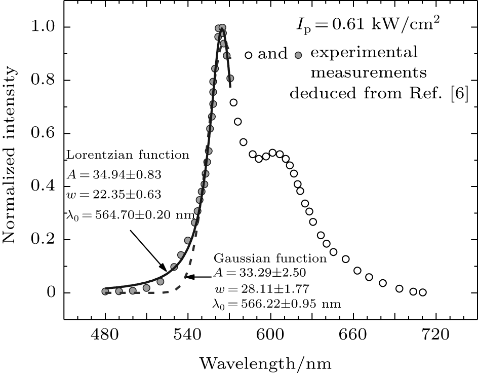
Fig. 6. Normalized experimental measurements of IASE versus wavelength for Ip = 0.61 kW/cm2 reported in Ref. [6]. The fittings to a Gaussian function and a Lorentzian function show that the intensity distribution favors a Lorentzian function at low input intensity.

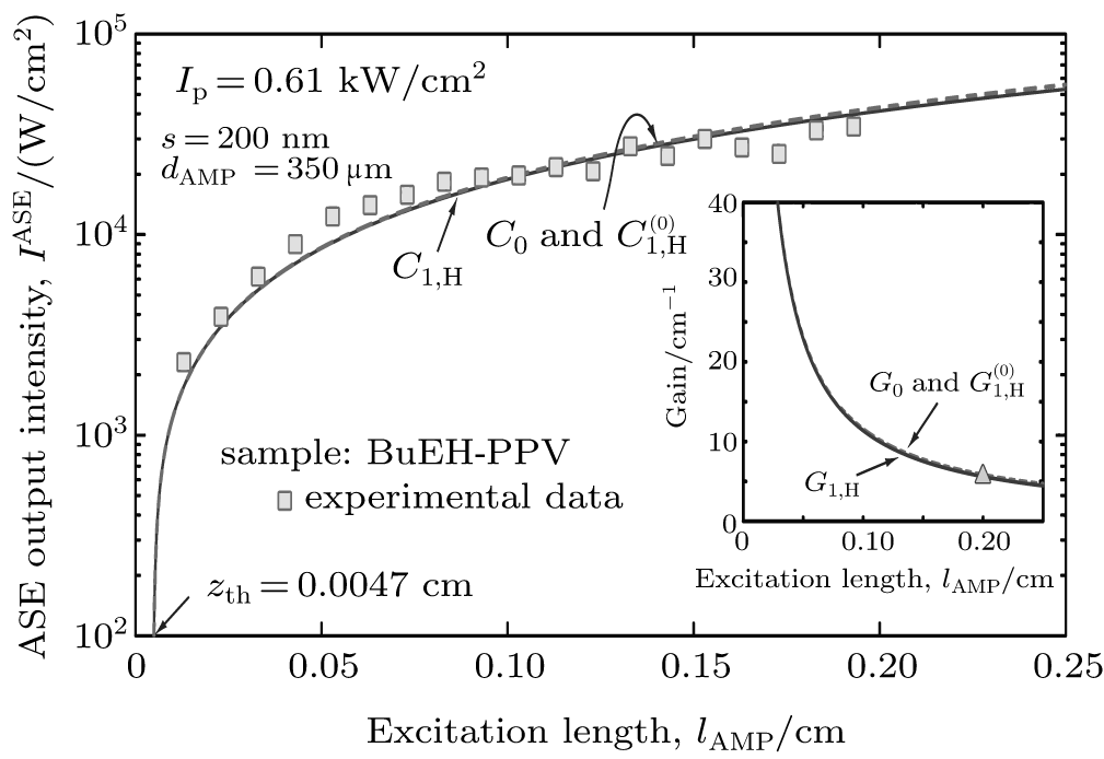
Fig. 7. Calculated ASE intensity corresponding to Ip = 0.61 kW/cm2 input intensity for μ = 0 and μ = 1 solutions shown by the C0, C1, H, and . The inset shows the corresponding gain shown by the G0, G1, H and , where for the condition, both intensity and gain profiles are overlapped. For lAMP = 0.2 cm, (△ ) is calculated. Experimental data are deduced from Ref. [6].
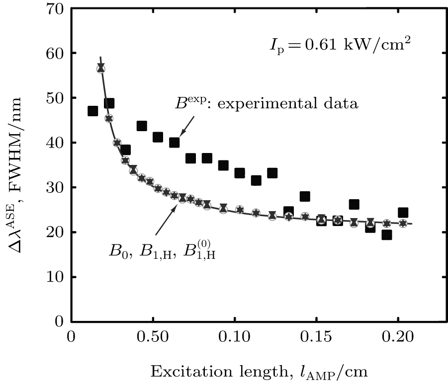
Fig. 8. Plots of the calculated ASE bandwidth, shown by the overlapped profiles of B0, B1, H, and versus excitation length. Bexp is the measured bandwidth.[6] This case refers to Ip = 0.61 kW/cm2, where is satisfied.

For observing that at a low Ip-value the Lorentzian distribution function maintains a Lorentzian frequency distribution along the whole excitation length of the sample, the ASE intensities for the excitation lengths of z = 0.20 cm and z = 0.01 cm are numerically calculated and the results are shown in Fig. 9. Again, fittings of a Lorentzian function and a Gaussian function to the calculated intensity profiles show that in both cases the frequency distributions favor a Lorentzian function. Thus, it is shown that by different approaches of using experimental measurements, as indicated in Ref. [6] and numerical calculations, a homogeneously broadened transition is involved in the light– matter interaction for the BuEH-PPV sample at different pump intensities. Figures 6 and 5(c) show that by increasing Ip from Ip = 0.61 kW/cm2 to 5.2 kW/cm2, the peak of the IASE shifts from 564.70 nm to 562.55 nm, i.e., it is blue-shifted. This behavior has also been shown by experimental graphs in slab organic crystals in the study of two-photon pumped ASE.[27] Here, regardless of the frequency shift, the effect of the pump intensity on the intensity behavior on switching from the Lorentzian distribution to the Gaussian distribution when the pump intensity increases is also explained by the proposed approach.

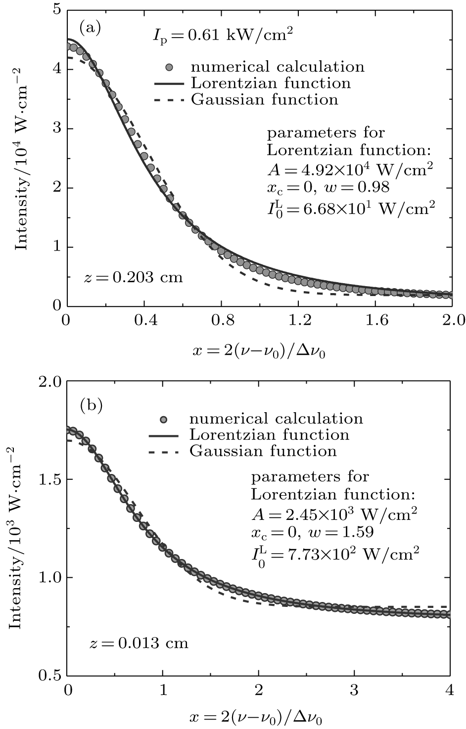
Fig. 9. The numerical calculation for the ASE intensity versus normalized frequency offset x = 2(ν ν 0)/Δ ν 0 for Ip = 0.61 kW/cm2 at: (a) z = 0.203 cm, and (b) z = 0.013 cm. Both profiles show that the intensity distributions favor Lorentzian functions at large, as well as, short distances.

4.3. D-broadening: calculation of Ip = 4.1 kW/cm2

In order to complete our analysis on the BuEH-PPV sample, the numerical calculations are also carried out on the assumption that the line is inhomogeneously broadened. In this case, the calculation results of bandwidth and gain coefficient have not explained the experimental measurements correctly.

To observe the results corresponding to the D-broadening, in Fig. 10 the ASE intensity versus lAMP is depicted. C1, D and correspond to the case where the saturation is included in the rate equation (i.e., μ = 1/2) and μ = 0 is used, when gain parameters from the μ = 1/2 solution are used. For the calculation , , s = 200 nm, and dAMP = 350 μ m for Ip = 4.1 kW/cm2 are used. This calculation gives zsat = 0.0871 cm, and zth = 0.0045 cm. Gain parameters for D-broadening are m′ = 35 cm− 1, , and b = 0.05 cm− 1. Although, apparently, the IASE behavior in this case is similar to that in Fig. 1, but with the deduced gain parameters we observe that the calculated gain-profiles are lower than expected. The calculated gain profiles corresponding to D-broadening lines are shown in the inset of Fig. 10. The and G1D, are the profiles corresponding to the unsaturated and saturated solutions, respectively. For lAMP = 0.2 cm, turns out to be 43.50 cm− 1, which is ∼ 1/2 of that calculated for H-broadened line (we remember that for Ip = 4.1 kW/cm2, , and even equation (1) gives 62 cm− 1). The is also calculated to be 12.39 cm− 1, which is higher than that of the H-broadened line (8.28 cm− 1). In Fig. 11 the calculated results corresponding to the ASE bandwidth for the μ = 1/2 solution are given. The B1, D and show the bandwidth behaviors for the saturated and unsaturated conditions, respectively while corresponds to the analytical solution given by Eq. (27). All the calculated ASE bandwidths are higher than the measurements as shown by the Bexp-profile in this figure, thus they can be rejected. Finally, with these calculations we confirm that the homogeneously broadened transition is responsible for the interaction. Our arguments in this respect are that the calculated ASE intensity and bandwidth profiles are consistent with those obtained from the measurements.

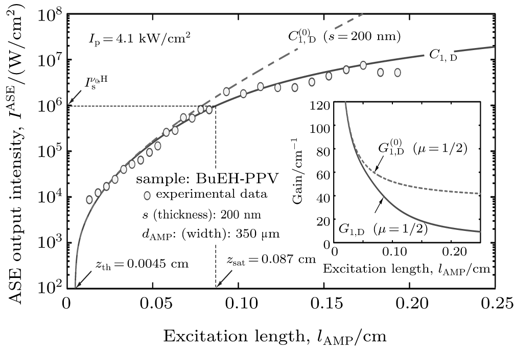
Fig. 10. Plots of the calculated ASE intensity for D-broadened line-shape for saturated C1, D- and unsaturated . The inset shows the calculated gain profiles for the unsaturation and saturation (G1, D-profile) conditions. For lAMP = 0.2 cm, is calculated to be 43.50 cm− 1, which is much lower than expected. Thus, the D-broadened line is not able to explain the ASE behavior.
Fig. 11. ASE band width calculations for saturated and unsaturated conditions, B1, D and ; and the analytical solution, , using Eq. (27). The calculated bandwidths for all three cases are higher than the values corresponding to measurements, shown by the Bexp-profile.

4.4. Results of gain calculations

According to the measurements appearing in Ref. [6] and the introduced model for data analysis, as given here, we calculate the gain parameters, unsaturated and saturated gain coefficients for Ip = 4.1, 2.2, 1.2, 0.61 kW/cm2. By referring to Fig. 12, in addition to introducing the plot of the unsaturated gain coefficient versus Ip as indicated in Ref. [6] using Eq. (1), the profiles of versus Ip, m′ versus Ip, and the saturated gain coefficient versus Ip in the present work are also given in this figure. We observe that and the m′ -parameters are linearly related to Ip with excellent linear fittings in the whole range of the given input intensity. A rough estimation of applying Eq. (1) to explaining the gain coefficient at low Ip, is also indicated in this figure. Thus, we are convinced that the plots of versus Ip and m′ versus Ip are linear. The calculated saturated gain coefficient, gν 0, versus Ip is also given in this figure, showing that at low values of the input intensity Ip, the system is not saturated, so we have . By increasing Ip, the value of gν 0 starts to increase, and after passing a maximum at Ip ≈ 1.2 kW/cm2, it decreases at high values of Ip. In fact, gν 0 refers to the net saturated gain coefficient. In Ref. [6], the measurement of IASE versus Ip shows that the corresponding plot has a change of slope at Ip ≈ 1.2 kW/cm2 that cannot be considered as a coincidence with the value of Ip corresponding to the measured peak of the gν versus Ip profile.

Fig. 12. Behaviors of the m′ deduced parameter and gain coefficient versus input intensity Ip. Gain parameter , and gain coefficients versus Ip, shown by (◯ ), (△ ), and (◊ ) symbols respectively; (■ ) refers to the analysis made using Eq. (1).[6]

By using Fig. 12, if we let

where α p and β p are constants, then equation (3) shows that for under the pumping condition, we can write

where z = lAMP = 0.2 cm, i.e., the total excitation length is used for this analysis. and are the -values of these quantities at the pump intensity. If we let

then, we observe that equation (36) is simplified into

which is true for the present analysis, as according to Table 1, and b remain constant in the analysis that has been made. Equation (37) shows that Γ p > α p, and also according to Eqs. (35) and (38), both and in the plots of and versus Ip have the same slope value of β p. If we use , we can also confirm that is linearly related to Ip. We may also notice from Fig. 12 that Ip = 1.2 kW/cm2 corresponds to the peak of versus Ip. It is seen that, as mentioned earlier, the m′ -parameter in this analysis, carries both saturation and pumping effects in the present experimental conditions.

5. Conclusions

In this work, the ASE in a planar waveguide BuEH-PPV sample of 2 mm in length, pumped by a laser pulse of 0.34 kW/cm2 to 5.2 kW/cm2, is investigated. For this purpose a model of geometrically dependent gain coefficient and the intensity rate equation are used to explain the ASE intensity behavior and bandwidth reduction for the pumped sample. It is shown that the system is homogeneously broadened with a Lorentzian frequency distribution, which at high input intensity switches smoothly to a Gaussian frequency distribution. That is, when the zzsat condition is satisfied, the distribution is a pure Gaussian function. At the low input intensity, on the other hand, the distribution behaves as a Lorentzian frequency function, because the experimental conditions have not reached the saturation. This corresponds to the zzsat condition. By analyzing the measured ASE intensity and bandwidth, the unsaturated and saturated gν 0 gain coefficients are determined and the corresponding plots of and gν 0 with respect to pump intensity, Ip are introduced. The D-broadening mechanism has also been examined by the analytical and numerical calculations, and their inconsistency with the measurements is confirmed. Thus, we are convinced that in this specific example, the transition line follows the homogeneous broadening mechanism. The GDGC model has already shown its potential for explaining the ASE behaviors in gas lasers of long excitation lengths. Here, its successful application of the model to solid organic materials proves further that the GDGC model, regardless of the pumping mechanism, gives a suitable method to be used in small-sized media. The mathematical approach made in this work confirms the validity of the GDGC model, where the proposed model explains the reported high values of gain coefficients in small-sized media. In general, with our present understanding of the GDGC model, due to the presence of the z-dependent power loss introduced in the intensity rate equation, the approach gives a powerful method of analyzing and explaining the ASE behaviors in excited laser media in the pulsed mode of operation.

Reference
1 Peters G I and Allen L 1971 J. Phys. A: Math. Gen. 4 238 DOI:10.1088/0305-4470/4/2/009 [Cited within:1]
2 Allen L and Peters G I 1971 J. Phys. A: Math. Gen. 4 377 DOI:10.1088/0305-4470/4/3/015 [Cited within:1] [JCR: 1.577]
3 Casperson L W and Yariv A 1972 IEEE J. Quantum Electron. QE-8 80 [Cited within:3]
4 Casperson L W 1977 J. Appl. Phys. 48 256 DOI:10.1063/1.323367 [Cited within:1] [JCR: 0.71]
5 Pert G J 1994 J. Opt. Soc. Am. B 11 1425 DOI:10.1364/JOSAB.11.001425 [Cited within:1] [JCR: 2.21]
6 McGehee M D, Gupta R, Veenstra S, Miller E K, Díaz-García M A and Heeger A J 1998 Phys. Rev. B 58 7035 DOI:10.1103/PhysRevB.58.7035 [Cited within:11]
7 Park J Y, Srdanov V I, Heeger A J, Lee C H and Park Y W 1999 Synthetic Met. 106 35 DOI:10.1016/S0379-6779(99)00032-6 [Cited within:1] [JCR: 2.109]
8 Zhang B, Hou Y B, Teng F, Lou Z D, Liu X J, Hu B and Wu W B 2011 Chin. Phys. B 20 054208 DOI:10.1088/1674-1056/20/5/054208 [Cited within:1] [JCR: 1.148] [CJCR: 1.2429]
9 Zhang B, Hou Y B, Teng F, Lou Z D, Liu X J, Hu B and Wu W B 2011 Chin. Phys. B 20 077803 DOI:10.1088/1674-1056/20/7/077803 [Cited within:1] [JCR: 1.148] [CJCR: 1.2429]
10 Xie W, Li Y, Li F, Shen F and Ma Y 2007 Appl. Phys. Lett. 90 141110 DOI:10.1063/1.2720298 [Cited within:1] [JCR: 3.794]
11 Wang H Y, Dou X M, Ni H Q, Niu Z C and Sun B Q 2014 Acta Phys. Sin. 63 021801(in Chinese) [Cited within:1] [JCR: 1.016] [CJCR: 1.691]
12 Samuel I D W and Turnbull G A 2007 Chem. Rev. 107 1272 DOI:10.1021/cr050152i [Cited within:1] [JCR: 41.298]
13 Calzado E M, Boj P G and Díaz-García M A 2010 Int. J. Mol. Sci. 11 2546 DOI:10.3390/ijms11062546 [Cited within:1] [JCR: 2.464]
14 Svelto O 2010 Principles of lasers5th edn. Berlin Springer [Cited within:6]
15 Yariv A and Leite R C 1963 J. Appl. Phys. 34 3410 DOI:10.1063/1.1729206 [Cited within:1] [JCR: 0.71]
16 Leonard D A 1965 Appl. Phys. Lett. 7 4 DOI:10.1063/1.1754241 [Cited within:1] [JCR: 3.794]
17 Kühnle G, Teubner U and Szatmári S 1990 Appl. Phys. B 51 71 [Cited within:1] [JCR: 1.782]
18 Hariri A, Jaberi M and Ghoreyshi S 2008 Opt. Commun. 281 3841 DOI:10.1016/j.optcom.2008.03.055 [Cited within:1] [JCR: 1.438]
19 Fitzsimmons W A, Anderson L W, Riedhauser C E and Vrtilek J M 1976 IEEE J. Quantum Electron. QE-12 624 [Cited within:1]
20 Sarikhani S and Hariri A 2010 Opt. Commun. 283 118 DOI:10.1016/j.optcom.2009.09.071 [Cited within:1] [JCR: 1.438]
21 Hariri A and Sarikhani S 2011 Opt. Commun. 284 2153 DOI:10.1016/j.optcom.2010.12.092 [Cited within:2] [JCR: 1.438]
22 Hariri A and Sarikhani S 2012 Opt. Lett. 37 1127 DOI:10.1364/OL.37.001127 [Cited within:3] [JCR: 3.385]
23 Hariri A and Sarikhani S 2014 Laser Phys. Lett. 11 015003 DOI:10.1088/1612-2011/11/1/015003 [Cited within:3] [JCR: 7.714]
24 Sarikhani S and Hariri A 2013 Opt. Commun. 286 251 DOI:10.1016/j.optcom.2012.08.040 [Cited within:1] [JCR: 1.438]
25 Hariri A and Sarikhani S 2014 Opt. Commun. 318 152 DOI:10.1016/j.optcom.2013.12.071 [Cited within:1] [JCR: 1.438]
26 Yariv A 1998 Quantum Electronics3rd edn. New York Wiley [Cited within:2] [JCR: 0.823]
27 Fang H H, Chen Q D, Ding R, Yang J, Ma Y G, Wang H Y, Gao B R, Feng J and Sun H B 2010 Opt. Lett. 35 2561 DOI:10.1364/OL.35.002561 [Cited within:2] [JCR: 3.385]