

Simulation study on characteristics of long-range interaction in randomly asymmetric exclusion process*
[Zhao Shi-Boa) , Liu Ming-Zhea), b)†  , Yang Lan-Ying
b) ]
, Yang Lan-Ying|
|


†Corresponding author. E-mail: liumz@cdut.edu.cn
*Project supported by the National Natural Science Foundation of China (Grant Nos. 41274109 and 11104022), the Fund for Sichuan Youth Science and Technology Innovation Research Team (Grant No. 2011JTD0013), and the Creative Team Program of Chengdu University of Technology.
In this paper we investigate the dynamics of an asymmetric exclusion process on a one-dimensional lattice with long-range hopping and random update via Monte Carlo simulations theoretically. Particles in the model will firstly try to hop over successive unoccupied sites with a probability q, which is different from previous exclusion process models. The probability q may represent the random access of particles. Numerical simulations for stationary particle currents, density profiles, and phase diagrams are obtained. There are three possible stationary phases: the low density (LD) phase, high density (HD) phase, and maximal current (MC) in the system, respectively. Interestingly, bulk density in the LD phase tends to zero, while the MC phase is governed by α, β, and q. The HD phase is nearly the same as the normal TASEP, determined by exit rate β. Theoretical analysis is in good agreement with simulation results. The proposed model may provide a better understanding of random interaction dynamics in complex systems.
The totally asymmetric simple exclusion process (TASEP) is an interacting particle system originally introduced by MacDonald in 1968[1] and has become a default stochastic model for transport phenomena. TASEP is a one-dimensional lattice model in which particles move unidirectionally with hard-core exclusion (that is, each site can be occupied by at most one particle at any given time). A large number of articles have been published on TASEP in physics, mathematics, and biology literature, [2– 24] such as gel electrophoresis, [4] protein synthesis, [5, 6] mRNA translation, [7] motion of molecular motors along cytoskeletal filaments, [8] and the depolymerization of microtubules by special enzymes, [9] as well as vehicular traffic problems.[10, 11]
Most of the TASEP models have been focused on one-dimensional lattices. Recently, the quasi-one-dimensional TASEP models considering long-range hopping have received much attention, such as in Refs. [12], [14], and [16]. The long-range hopping may be inspired by (i) a shortcut path in vehicular traffic, (ii) a quick end-to-end data package transformation inside a buffer in a router, and (iii) a plaything slingshot or catapult which is used to propel small stones in reality. Thus, various long-range hopping models have been presented. In Ref. [12], long-range hopping means that particles may jump any distance l ≥ 1 with the probability l− (1+ δ ), while long-distance jump in Ref. [14] is predetermined and runs on a hierarchical network. Authors reported that the particle– hole symmetry is broken and no maximum-current phase is observed.[14] The TASEP with a shortcut in its bulk has also been studied by Yuan et al.[16] We note that the shortcut, i.e., the position of long-range hopping, is fixed in Ref. [16]. However, the position of long-range hopping may be various in some cases such as in motor-protein transport. In the statistical physics perspective, motor-protein transport can be modelled by particles travelling larger distances along a one-dimensional filament.[19] In order to investigate the jumping dynamics of motor proteins for a better understanding of the motor-protein motion mechanism, this paper presents a simplified model, that is, we just allow a motor protein jumping as far as possible at the first movement, and then moving one step with hard-core exclusion.
Inspired by motor-protein transport, this paper studies a one-dimensional random access model using the totally asymmetric simple exclusion process (TASEP) with long-range hopping and random update. With regard to random transport networks, the hopping probabilities of particles may reflect the ability of particle’ s hopping expectation. The entry and exit in the TASEP models may correspond to the source and the destination of random access. This paper is organized as follows. In Section 2, the model is described. In Section 3, we discuss the results obtained from Monte Carlo simulations and theoretical analysis. We give conclusions in Section 4.
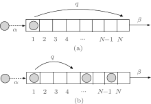
A one-dimensional TASEP with long-range hopping and random update is illustrated in Fig. 1. The model is defined in a one-dimensional lattice of N sites with open boundary conditions. N is the system size of the model and q represents the long-range hopping probability. Particles are assumed to move from the left end to the right end. At the entrance site, a particle can enter the system with rate α provided the site is empty. At the exit site, a particle can leave the system with rate β . An occupation variable, τ i, is defined to denote the state of the i-th site (1 ≤ i ≤ N). τ i = 1 (or τ i = 0) means that the i-th site is occupied (or empty). The following rules are applied to a randomly chosen site: i) If τ 1 = 1 and τ j = 0 (1 < j ≤ N), a particle at site 1 can hop to site j with probability q as far as possible once the successive sites from site 2 to site j − 1 are unoccupied (see Figs. 1(a) and 1(b)); ii) If τ i = 1 and τ i + 1 = 0 (1 ≤ i ≤ (j − 1)), a particle at site i can move to site (i + 1) with probability 1. That is, a particle can only move forward one site in each time step within the lattice; iii) If τ i = 1 and τ i + 1 = 1, a particle at site i does not move forward. An obvious difference between our model and other TASEP models is that particles in other TASEP models will firstly arrive at the first site and then move forward one site. However, in our model particles at site 1 will firstly try to hop to the last site, site N with probability q. If the last site is occupied, particles will hop to site (N − 1) with probability q, and so on. The first site could be occupied only when the system is congested.
 | Fig. 1. Illustrations of the corresponding one-dimensional TASEP with long-range hopping and random update. q represents the long-range hopping probability. The filled circles mean particles. Only particles at the first site can hop over successively unoccupied sites. Panels (a) and (b) show possible long-range hoppings. |
Monte Carlo simulations are performed here to investigate the system properties. The system size is assumed to be N = 1000. Steady-state density profiles and currents are obtained by averaging 109 sampling. The system firstly runs 108 time steps to let the transient time out.
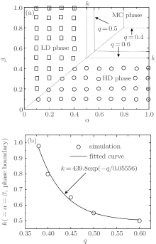
The phase diagram of our model is shown in Fig. 2. It is found that there are some similarities and differences compared with the normal TASEP. The main similarity is that both phase diagrams include three phases, that is, the phase structure does not change. The main difference is that the phase region in our model changes with the value of q. With the increase of q, the MC phase region expands while the LD and HD phase regions shrink in our model. In the simulations, it is found that when q < 0.36, there is no MC phase. Here, the MC phase means that the bulk density is equal to 0.5, while the current is equal to 0.25. When q = 0.36, the MC phase exists in an extreme region with α = 1 and β = 1. Interestingly, when q ≥ 0.6, the phase diagram in our model will revert to the normal TASEP (see Fig. 2(b)). However, the density profiles and currents in the LD and HD phases may be different from those of the normal one. To study the phase boundaries among the LD, HD, and MC phases, we obtained the fitted curve based on 5 simulations of different q values (see Fig. 2(c)). The fitted curve can be written as

where q ∈ [0.36, 0.6], k = α represents the phase boundary between the LD and MC phases, and k = β corresponds to the phase boundary between the HD and MC phases. q is the hopping probability. Using Eq. (1), one can calculate the phase boundary and get the phase diagram of the system according to the hopping probability q.
 | Fig. 2. Phase diagrams for TASEP with long range hopping under random update. (a) phase diagrams for q = 0.4, 0.5, 0.6; (b) fitted curve for phase boundary. |
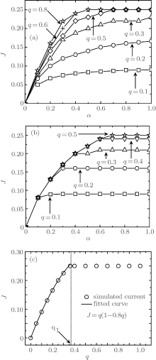
Steady-state currents in the three phases are simulated, as shown in Fig. 3(a)– 3(c). In the LD phase, the current depends upon α and q. Thus, the current increases with the increase of α or q. When α increases to a critical value, q dominates the currents. In the HD phase, exit probability β determines the current. In Fig. 3(c), we simulate the current at the extreme case of α = β = 1.0. It is found that the current increases with the increase of q when q ≤ q1 (q1 = 0.36). Once q ≥ q1, the current reaches the maximum value, 0.25. The fitted curve J = q(1 − 0.8q) describes well the relationship between the current J and hopping probability q for q ∈ [0, 0.36].
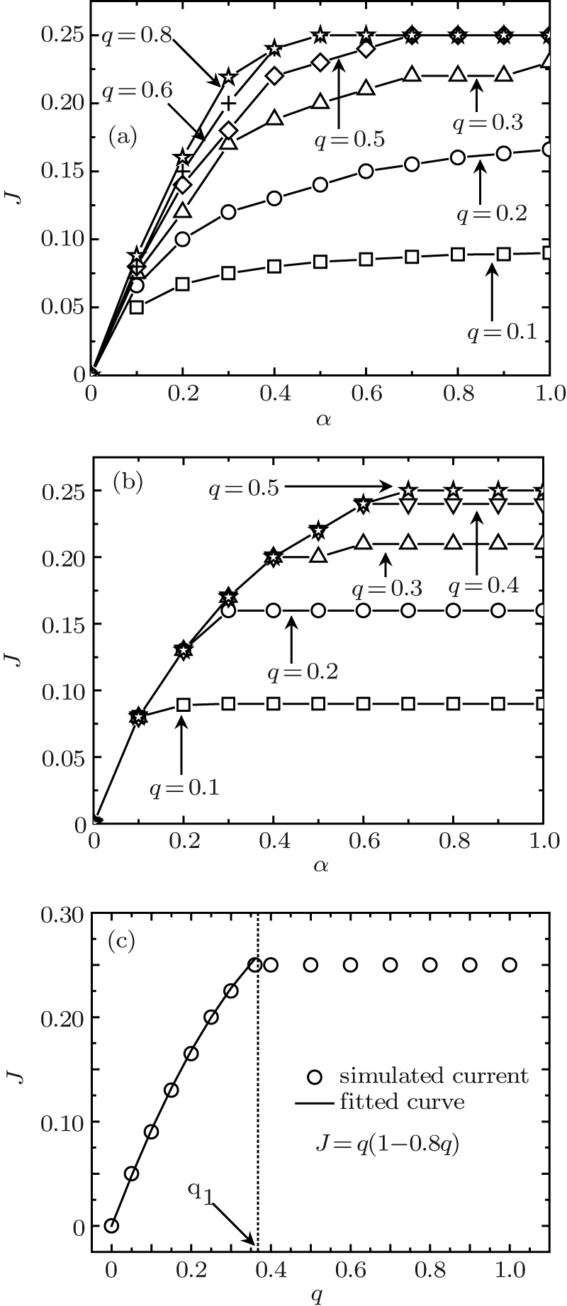 | Fig. 3. Steady-state currents in the system for various q. (a) β = 0.4; (b) β = 0.8; (c) α = β = 1.0. |
We then investigate the density profiles in the LD and HD phases (see Fig. 4(a)– 4(b)). In the LD phase, particles leave the system much more efficient than they are inserted, which leads to particles having little chance to fall in the bulk except near the exit boundary. Consequently, the bulk density is expected to be flat and almost zero, while it gradually increases upon approaching the right end. In the HD phase, the entrance of particles is more effective than the removal. Accordingly, a shock is a back propagation to the left end. It can be seen that in our model the first site is the last site that particles hop to, which explains why the density at the first site is always larger than other sites. Conversely, a particle firstly arrives at the first site and then moves forward in other TASEP models.
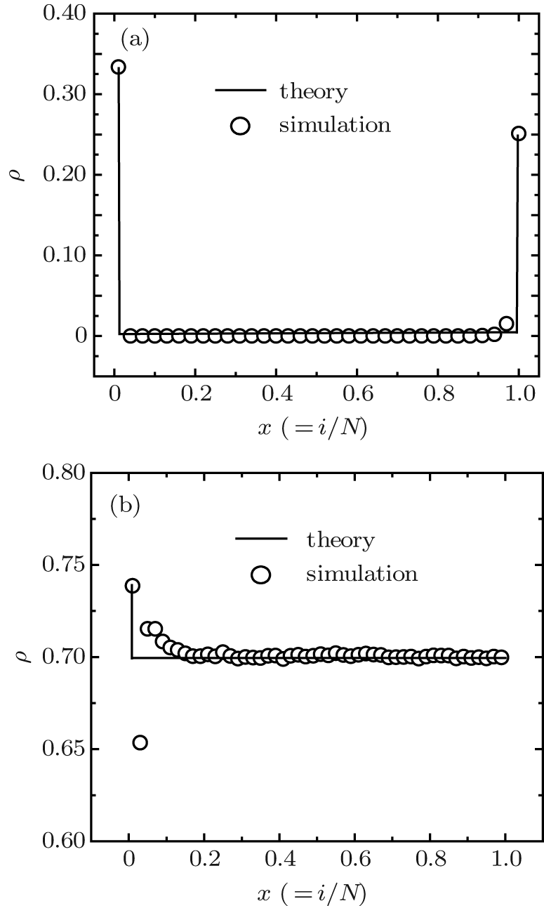 | Fig. 4. Simulation and theoretical results. (a) Steady-state density profiles in the LD phase for α = 0.3, β = 0.8, and q = 0.6; (b) Steady-state density profiles in the HD phase for α = 0.8, β = 0.3, and q = 0.6. |
Figure 5(a) shows phase transitions between the LD and HD phases under random update. When α = 0.1 (β = 0.1 and q = 0.5), the system is in the LD phase. With the increase of α , densities near the right boundary gradually increase. When α = 0.11, the system is in the critical state, that is, the LD and HD phases coexist. Once α increases continuously, e.g., α ≥ 0.115, the system transfers to the HD phase. The phase transitions under parallel update have been simulated, as shown in Fig. 5(b). It can be seen that figures 5(a) and 5(b) are quite similar, but the obvious difference is that the transition in our model is a convex curve, while it is a notching curve in the case of parallel update procedure.
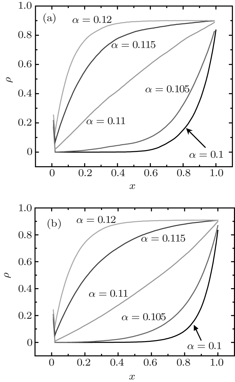 | Fig. 5. Phase transition between LD and HD density profiles in Monte Carlo simulations. The parameters are: β = 0.1 and q = 0.5. (a): Random update procedure; (b) parallel update procedure. |
The starting point of analyzing this model is the rule of current conservation through the system. We thus have

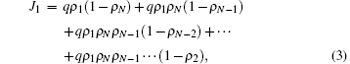
where JL corresponds to the entry current; JR corresponds to the exit current, and J1 corresponds to the current of particles with long-range hopping at site 1. In Eq. (3), qρ 1(1 − ρ N) represents the current from site 1 to site N, while qρ 1ρ N(1 − ρ N− 1) calculates the current from site 1 to site (N − 1) once site N is occupied, and so on. Equation (3) can be expanded as
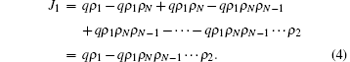
Since q < 1 and ρ i < 0.5 (1 < i < N) in the LD phase, the item qρ 1ρ Nρ N− 1· · · ρ 2 will tend to be zero. Thus, equation (4) can be simplified to be

Combining with Eqs. (2) and (5), we solve

It is found that the LD phase is controlled by α and q. In the HD phase, the long-range hopping rule makes particles have little probability to jump to site N, thus the HD phase is only determined by exit rate β . We thus have

Accordingly, in the HD phase one can obtain

The phase boundary between the LD phase and the HD phase can be determined by the following consideration. At the boundary, currents in the LD and HD phases are the same. That is, β (1 − β ) = qα /(q+ α ) which is equivalent to

Since α ≤ 1, equation (9) should satisfy
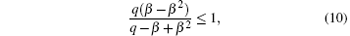
which leads to

One-dimensional totally asymmetric exclusion process (TASEP) with long-range hopping and random update is numerically investigated in this paper. The model is relevant to random access over networks. A reduced hopping probability q may represent available access. In our model, particles will firstly try to hop to the last site, which is the main difference from other TASEP models. Computer simulations are carried out to exhibit three possible stationary phases (LD, HD, and MC phases) in the system. The current in the LD phase is determined by both q and α and the bulk density tends to zero. Interestingly, the HD phase is the same as that of the normal TASEP. With the increase of q, the LD and HD phase regions shrink, while the MC phase region expends. The numerical fittings for current and phase boundary are performed. An integrated picture of the system is obtained. In the model, particles are just assumed to have one hopping. In reality, multiple hoppings are possible. The dynamics of such a system is more interesting and under investigation at present. The results will be reported later.
| 1 |
|
| 2 |
|
| 3 |
|
| 4 |
|
| 5 |
|
| 6 |
|
| 7 |
|
| 8 |
|
| 9 |
|
| 10 |
|
| 11 |
|
| 12 |
|
| 13 |
|
| 14 |
|
| 15 |
|
| 16 |
|
| 17 |
|
| 18 |
|
| 19 |
|
| 20 |
|
| 21 |
|
| 22 |
|
| 23 |
|
| 24 |
|