

Principal resonance response of a stochastic elastic impact oscillator under nonlinear delayed state feedback*
[Huang Dong-Meia), b) , Xu Weia)†  , Xie Wen-Xian
a), b) , Han Quna) ]
, Xie Wen-Xian|
|


†Corresponding author. E-mail: weixu@nwpu.edu.cn
*Project supported by the National Natural Science Foundation of China (Grant Nos. 11172233, 11302170, and 11302172).
In this paper, the principal resonance response of a stochastically driven elastic impact (EI) system with time-delayed cubic velocity feedback is investigated. Firstly, based on the method of multiple scales, the steady-state response and its dynamic stability are analyzed in deterministic and stochastic cases, respectively. It is shown that for the case of the multi-valued response with the frequency island phenomenon, only the smallest amplitude of the steady-state response is stable under a certain time delay, which is different from the case of the traditional frequency response. Then, a design criterion is proposed to suppress the jump phenomenon, which is induced by the saddle-node bifurcation. The effects of the feedback parameters on the steady-state responses, as well as the size, shape, and location of stability regions are studied. Results show that the system responses and the stability boundaries are highly dependent on these parameters. Furthermore, with the purpose of suppressing the amplitude peak and governing the resonance stability, appropriate feedback gain and time delay are derived.
In an elastic impact (EI) system, as a kind of non-smooth system, it is assumed that the impacting bodies are elastic with either linear or nonlinear stiffness and damping. As is well known, EI systems are often encountered in the engineering fields, such as cantilever systems, large-scale structures, and rotor systems with clearances. Because of the existence of impacts, many interesting phenomena can be found in this system.[1– 6] For example, the single or normal mode characteristic of the forced frequency response of a system with multiple clearance has been found in Ref. [1]. Grazing chaos and bifurcation of a forced cantilever system with impacts have been investigated in Refs. [2] and [3]. The global dynamic behavior of the EI system with one random parameter has been presented in Ref. [4]. However, the present research involving this system mainly focuses on the deterministic EI system. There are a few conclusions about the stochastic EI system, especially with time delay feedback control.
As is well known, time delays, which usually exist in the feedback of controlled physical, mechanical or electrical systems, are always unavoidable due to the time spent in measuring system states, calculating and executing the control forces, etc. On the one hand, additional time delays in the feedback path not only cause the transfer function of the controller to be modified, but also may induce the instability of the controlled system. On the other hand, time delays can be deliberately implemented to achieve better system behavior. Therefore, in the past two decades, a great deal of attention has been paid to study the dynamics of the delay controlled systems.[7– 25] Famous examples are presented by Hu et al.[7, 8] From the concept of the equivalent damping ratio, they proposed an appropriate choice of the feedback gains and time delays to enhance the control performance. Actually, most of the results focused on the smooth dynamic systems, and limited results are available for the non-smooth systems. Recently, Saha and Wahi[21] considered a linear time-delayed position feedback in controlling friction-induced vibration in a system on a moving belt with friction having hysteresis. A direct linear velocity feedback strategy is called a skyhook damping for the reason that in its “ off” state, the damping coefficient is relatively low, while in its “ on” state, it is relatively high. This may introduce a sharp increase in damping force and lead to a jerk in the acceleration response.[25] Thus, in order to overcome the disadvantage of a direct linear velocity feedback strategy, a nonlinear cubic velocity feedback has been used to explore the dynamics of a piecewise bilinear vibration isolation system.[22] Compared with the on-off skyhook damping, the feedback gain of the control strategy is a constant, and thus the jerk induced by the abrupt change of damping force can be avoided.
Motivated by the above findings, this study aims at gaining an insight into the dynamics of an EI system with time-delayed cubic velocity feedback subjected to stochastic excitation. The rest of this paper is organized as follows. In Section 2, a brief description of the stochastic EI system with time-delayed feedback is introduced. Then, based on the method of multiple scales, the steady-state responses and stability conditions are derived. In Sections 3 and 4, the effects of system parameters on the dynamic behaviors are revealed in deterministic and stochastic cases, respectively. The jump avoidance condition is given analytically. Finally, some conclusions are drawn from the present study in Section 5.
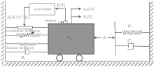
In this paper, the nonlinear oscillator considered here is a single degree-of-freedom system with an active vibration controller as shown in Fig. 1, which serves as the model for a wide range of EI systems in engineering practice. The corresponding differential equation of motion with time-delayed cubic velocity feedback is given as follows:[4]
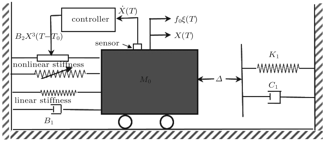 | Fig. 1. Sketch map of the elastic impact oscillator with an active vibration controller. |
where

is the elastic impact force with spring stiffness K1 and damping coefficient C1. It exists only when the impact happens. M0, K, B1, and C are the mass, linear stiffness coefficient, linear viscous damping coefficient, and nonlinear stiffness coefficient, B2 and δ denote the feedback gain and the designed time delay in the controller respectively.
By introducing the following non-dimensional parameters:

the following non-dimensional equation of motion is derived:
where


The stochastic excitation ξ (t) represents an ergodic narrow-band stochastic process with zero mean, and is governed by the following equation given by Wedig[26]

whereΩ is the center frequency, W(t) is the standard Wiener process with the intensity of γ .
The method of multiple scales will be extended to investigate the responses and its stability of system (2). For the necessity of the method of multiple scales, we may denote 

Then, the uniformly approximate solution of Eq. (4) is assumed to be in the form of

where T0 = t is a fast time scale and T1 = ε t is a slow time scale. By denoting the differential operators D0 = ∂ /∂ T0 and D1 = ∂ /∂ T1, we obtain

Substituting Eqs. (5) and (6) into Eq. (4) and comparing coefficients of ε with the same powers, we obtain the following equations:
Here, the statistical property of the standard Winner process

is used in the second expression of Eq. (7).
Denoting excitation frequency as Ω = 1 + ε σ (σ is the detuning parameter), considering the primary resonance of system (2), and according to Eq. (7), the general solution can be expressed as

where A = A(T1) and ϕ = ϕ (T1) are functions of the slow time scale.
Introducing new variables ψ (T0, T1) = T0 + ϕ (T1) and 
According to Eq. (2), F0(x0, D0x0) is a piecewise linear function. Using the periodic property of cosine function, the integral can be calculated in three intervals: [0, ψ 0], [ψ 0, 2π − ψ 0], [2π − ψ 0, 2π ], where ψ 0 corresponds to the phase of the discontinuity point in one period. Then, the Fourier coefficients of basic harmonic terms of F0(x0, D0x0) can be given as follows:
in which G = sin ψ 0 − Aψ 0.
In order to eliminate the secular term in Eq. (10), the right-hand side of Eq. (10) should not include the terms sin ψ and cos ψ , thus we have

Therefore, by solving Eq. (11) for the amplitude A(T1) and the phase η (T1), the lowest-order expansion of the solution can be written as

Firstly, the steady-state response of system (2) as γ = 0 is determined. In this case, according to Eq. (8), 

Therefore, the frequency response equation can be expressed as
Next, we examine the stability of the steady-state response by introducing the perturbation terms as

where A0 and η 0 are governed by Eq. (13), A1 and η 1 are perturbation terms.
Substituting Eq. (15) into Eq. (11) and neglecting the nonlinear terms, we can obtain the linearization modulation of Eq. (11) at A0 and η 0
where

By means of the characteristic equation of the coefficient matrix of Eq. (16) and the Routh– Hurwitz criterion, [27] the steady-state solutions of Eq. (11) are asymptotically stable if the following two inequalities hold simultaneously:

where
In fact, if N is negative, the corresponding steady-state solutions in Eq. (14) lose stability via a saddle node bifurcation, which means that the jump phenomenon could happen. In addition, the steady-state solutions associated with M2 − 4N < 0 are foci, while those associated with M2 − 4N > 0 are nodes. These points are stable (unstable) when M < 0 (M > 0). Actually, the stability boundary M indicates the critical condition that the signs of the real parts of both roots of the characteristic equation change. A change from negative real parts to positive real parts indicates the presence of a Hopf bifurcation. Therefore, the non-trivial solutions are stable if and only if the conditions M < 0 and N > 0 are satisfied.
In this part, the steady-state response of system (2) is discussed in the mean square sense as γ ≠ 0 but is sufficiently small. Let

in which A0 and η 0 are governed by Eq. (13), A11 and η 11 are the small perturbations.
Linearizing Eq. (11) at (A0, η 0) with respect to A and η , the following Itô stochastic differential equations can be obtained as
By combing the moment method and the property of

the first-order and second-order steady-state moments of A11 and η 11 can be obtained from Eq. (19) as follows:

where E(• ) denotes the mathematical expectation.
According to Eqs. (21) and (22), the necessary conditions for the existence of the second-order moments of the response are 


By using the Routh– Hurwitz criterion, [27] the non-trivial steady-state solution is asymptotically stable, when the following inequalities hold:
Combining Eqs. (18) and (21), the mean square steady-state response of system (2) is
In this section, we consider the dynamic response properties of the controlled EI system under deterministic excitation. The numerical simulations are performed by numerically integrating the time-delayed EI system using the fourth-order Runge– Kutta algorithm. Throughout our study, the parameters of system (2) are set as b = 0.06, c = 0.02, d = 0.01, k1 = 0.05, c1 = 0.02, f = 0.2, and ε = 0.1, unless otherwise stated.
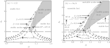
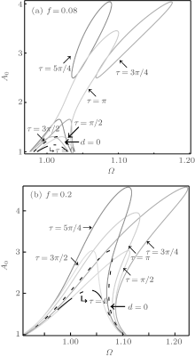
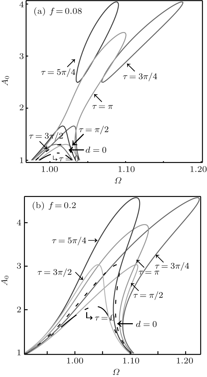
In Fig. 2, several frequency response curves defined by Eq. (14) are plotted for different values of time delay τ = π /2 and τ = 3π /4, respectively. The solid lines represent approximate analytical results by the multiple scale method. By comparing Fig. 2(a) with Fig. 2(b), it can be seen that the time delay can cause a great change in the frequency response. Specifically, for τ = π /2, M is negative in the Ω – A0 plane, thus, the shaded region (N < 0) covers all the unstable solutions. The solutions in the shaded region (M2 − 4N > 0) are stable nodes, while outside this region they are stable foci. However, as time delay increases such as τ = 3π /4 in Fig. 2(b), for larger f (f = 0.2), the frequency response curve is continuous with the apparent maximum. As f decreases, the left and right branches get closer to each other (f = 0.15). There exists a critical value f = 0.08575 (this shows up more clearly in Fig. 3), the frequency response curve is separated into two parts (as depicted for f = 0.08), which is called the frequency island. Furthermore, the steady-state solutions, which not only exist in the shaded region (N < 0) but also lie above the dash line (M = 0), are unstable. Hence, the frequency islands here are formed by two unstable solution branches, [27] which is different from the general case that the frequency islands are created by either two stable solution branches or at least one stable solution branch. Accordingly, the classification of the steady-state solutions is also presented in Fig. 2(b) when τ = 3π /4.
The numerical results are denoted by circles in Fig. 2 and the good agreement between numerical results and analytical ones can be found. Additionally, the steady-state response curves below the line A0 = 1 are the special case, which are derived in the degradation case, that is to say, the gap Δ is infinite, thus the value of the non-dimensional elastic impact force F0(x, ẋ ) is always zero.
 | Fig. 2. Steady-state responses versus excitation frequency (solid lines: analytical results; circles: numerical results). |
In Subsection 3.1, the existence of the jump phenomenon is indicated. Because of the undesirable and destructive effects of jumps in practical situations, it is important to find the condition required to avoid the jump.[28, 29] A jump can be avoided if it can be ensured that the frequency response of the system is unique. According to Eq. (14), the excitation frequency can be derived as follows:
where 
Differentiating both sides of Eq. (26) with respect to A0 and substituting dΩ /dA0 = 0 yield

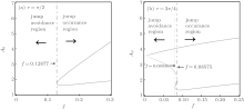
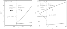
According to Eq. (27), figure 3 depicts the critical amplitude A0 as a function of excitation amplitude f when τ = π /2 and τ = 3π /4. As shown in Fig. 3(a) (τ = π /2), there is more than one point satisfying dΩ /dA0 = 0 for f > 0.12877, indicating the existence of a jump. When f < 0.12877, there is no critical amplitude, and therefore no jump. Hence, f = 0.12877 is the maximum and acceptable value of f in the practical design to avoid the jump. However, for the special case of τ = 3π /4 in Fig. 2(b), the critical amplitude A0 also presents particular features; it can be analyzed specifically in the following part by means of the frequency response curves.
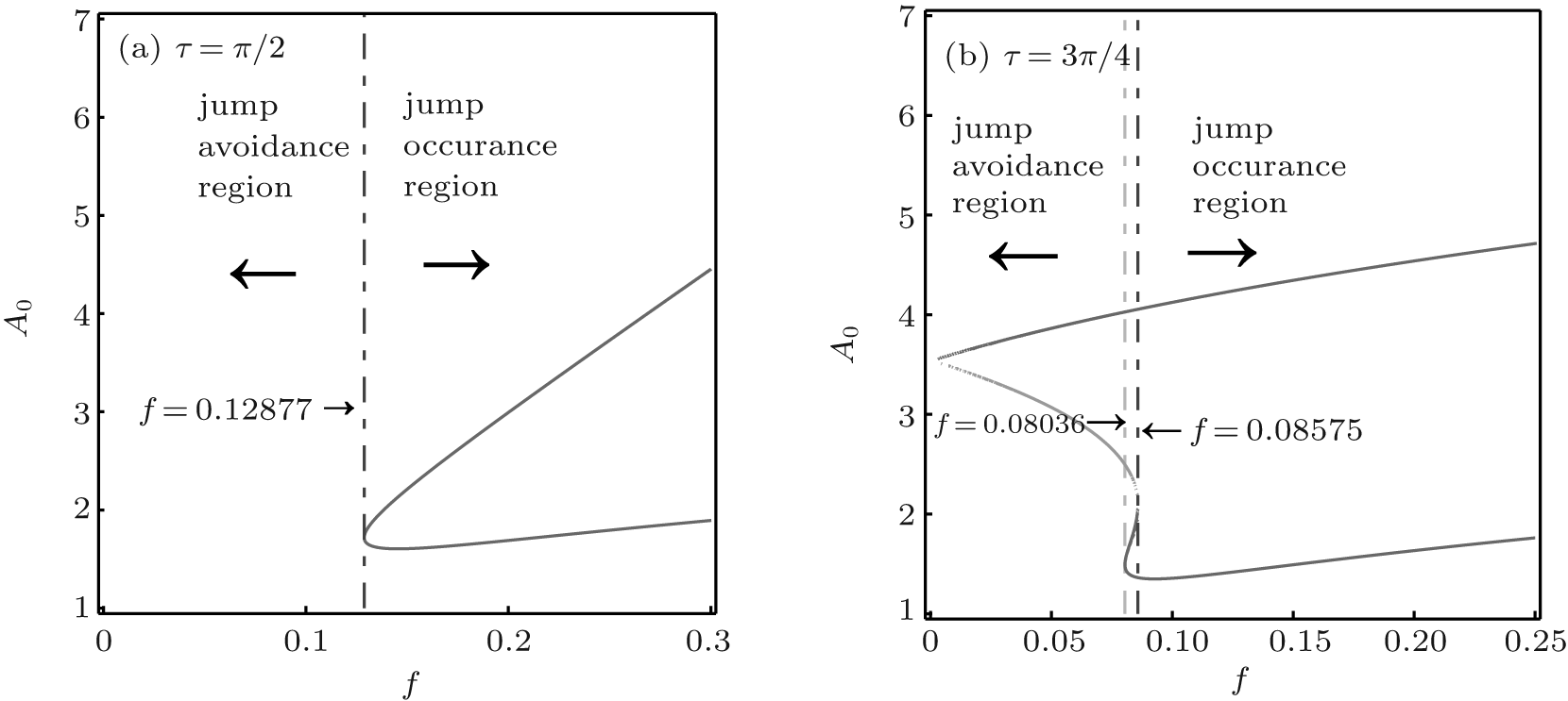 | Fig. 3. No-jump region indicating maximum acceptable values of excitation amplitude f. |
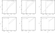
Obviously, as f > 0.08575 in Fig. 3(b), there are two points satisfying dΩ /dA0 = 0, which means the existence of a jump. Actually, f = 0.08575 is the critical amplitude for the continuous frequency response and the frequency island phenomenon; the cases of f = 0.0856 and f = 0.0858 are taken for examples, which are plotted in Figs. 4(a) and 4(b). Then, in the small interval of 0.08036 < f < 0.08575, there are four points satisfying dΩ /dA0 = 0. On the one hand, the branch of the frequency island of the lower amplitude part presents the jump phenomenon, therefore there are two points at which dΩ /dA0 = 0; on the other hand, the other two points come from the island, such as in the cases of f = 0.0856 and f = 0.085 shown in Figs. 4(b) and 4(c). When the excitation amplitude f < 0.08036, there remains only two points at which dΩ /dA0 = 0. In fact, two kinds of responses still exist: one is the case of f = 0.08 in Fig. 4(d), which is composed of the lower amplitude part and the higher amplitude part (the closed loop); the other one is for the case of f = 0.05 in Fig. 4(f) and there remains only the branch of the higher amplitude part. The gradual change process of the response can be seen from Figs. 4(d)– 4(f), and the lower branch disappears gradually with the decrease of f.
 | Fig. 4. Steady-state responses versus excitation frequency: (a) f = 0.0858; (b) f = 0.0856; (c) f = 0.085; (d) f = 0.08; (e) f = 0.06; (f) f = 0.05. (Solid lines: analytical results; dash– dot lines: vertical tangent). |
In this subsection the jump avoidance condition is derived and the effectiveness is also confirmed by comparing with the corresponding frequency response curves.
In view of the dominant factor of the damping in the EI system, therefore, the equivalent damping of the controlled nonlinear system is introduced.
Multiplying both sides of Eq. (14) with ε 2, equation (14) can be rewritten as
Therefore, the equivalent damping ratio can be defined as[7]

We only consider the positive velocity feedback, obviously, the extreme values of the damping ratio are

Therefore, when τ lies in [0, π /2] and [3π /2, 2π ], the following inequality is satisfied:

Note that b/2 − c1G0/2π A0 is the equivalent damping ratio of an uncontrolled system and 
 | Fig. 5. Comparison of frequency responses among the uncontrolled system (dot line), controlled system without time delay (dash– dot line), and controlled system with different values of time delays (solid lines). |
When τ lies in [π /2, 3π /2], we have

As a result, the equivalent damping value is even smaller than the equivalent damping of the uncontrolled system, thus, the response amplitude in the resonance region could rise compared with the uncontrolled system (Fig. 5).
Figure 5 shows the effect of time delay on the response amplitude in the range of [0, 2π ], which coincides with the variation of equivalent damping beq discussed in the above analysis.
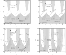
In this section, we focus on analyzing the effects of time delay and feedback gain on the steady-state response. The value of excitation frequency is fixed to be Ω = 1.05. Figure 6 shows the effects of time delay τ on the steady-state response under different values of feedback gain d.
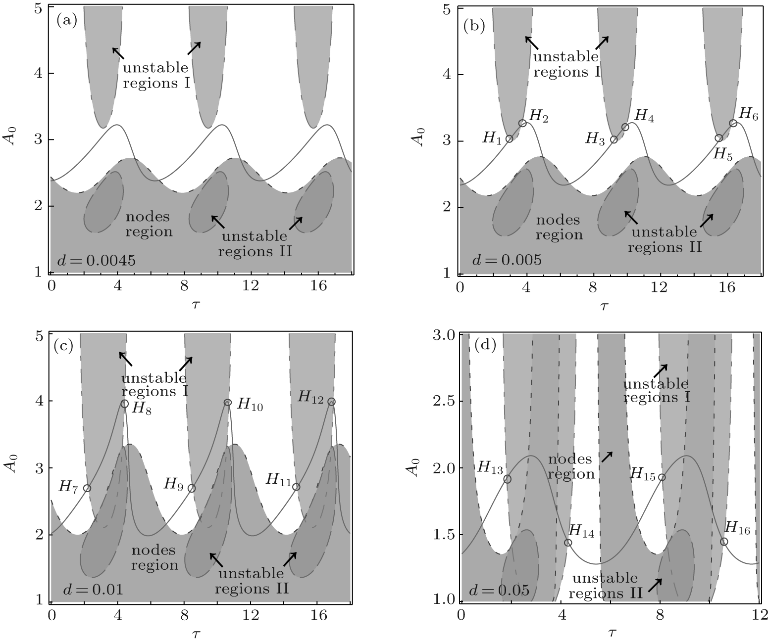 | Fig. 6. Effects of time delays on the steady-state responses and stability boundaries: (a) d = 0.0045; (b) d = 0.005; (c) d = 0.01; (d) d = 0.05. (Solid lines: steady-state response curves; dash and dash– dot lines: unstable boundaries; dot lines: nodes boundaries). |
As indicated in Fig. 6, shaded regions I and II present the unstable regions which are predicted by inequality (17). Obviously, when the value of feedback gain d is smaller (d = 0.0045 in Fig. 6(a)), the response curve lies outside the unstable region, which means that the steady-state solutions are stable everywhere in spite of different time delays. As feedback gain increases gradually, the size of the unstable region I increases and then there are some parts of the response curve which lie in the unstable region I (d = 0.005 in Fig. 6(b)). Moreover, from two independent parts (in Figs. 6(a) and 6(b)), the unstable regions I and II intersect with each other (in Figs. 6(c) and 6(d)) as feedback gain increases further. However, unstable solutions can be found only in unstable region I rather than unstable region II, actually, which is caused by the larger value of f.
For the classification of the steady-state solutions, it should be noted that steady-state solutions, which lie in unstable region II, are saddle points; while the steady-state solutions in the node region are nodes and outside this region they are foci. The boundaries of the unstable region I are the division lines for stable and unstable nodes and foci. In addition, the points in the boundaries of the unstable region I are Hopf bifurcation points, which are denoted by circles in Fig. 6.
The results in this subsection indicate that the size, shape, and location of stable and unstable regions depend on the system parameters and the feedback control gains.
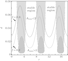
From the analysis in the previous sections, it can be found that high amplitude response suppression can be performed with appropriate time delays and feedback gains. In this part, we aim to find suitable feedback parameters which can give a stable steady-state response and reduce the peak amplitude.
Taking the peak amplitude A0 = 2 for example, the relation of time delay τ with feedback gain d can be derived from Eq. (14) and is presented by solid lines with f = 0.2 and f = 0.3 in Fig. 7. The regions above these two curves are the optional parameter regions corresponding to the peak amplitude smaller than 2. However, the whole parameter pairs do not satisfy the stability conditions above these curves. We can derive the stable boundaries from the stability condition (15), which are depicted with the dash– dot lines and dash lines, respectively.
 | Fig. 7. Design control parameter pairs (time delay and feedback gain) for suppressing the maximum amplitude; the shaded regions represent the unstable parameters regions. |
The results in this section suggest that the time delay and feedback gain can be used as a control switch to control the peak amplitude and stability of the steady-state responses.
In this section, we determine the effects of the noise term ξ (t) on the primary response in the case γ ≠ 0. For the simulation of narrow-band random noise, readers can refer to Refs. [30] by Shinozuka and Ref. [31] by Zhu.
In Fig. 8 the variations of mean response EA2 with Ω are shown as 
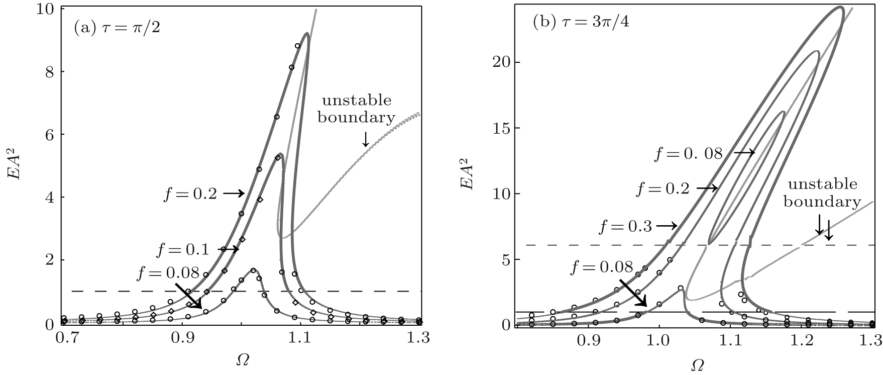 | Fig. 8. Mean square responses versus excitation frequency for  |
Then, according to the relation between the steady-state response and the mean square response, we can also derive the critical value of f for jump avoidance in the stochastic case as shown in Fig. 9, which also have the same characteristics as that for the deterministic case under small noise intensity.
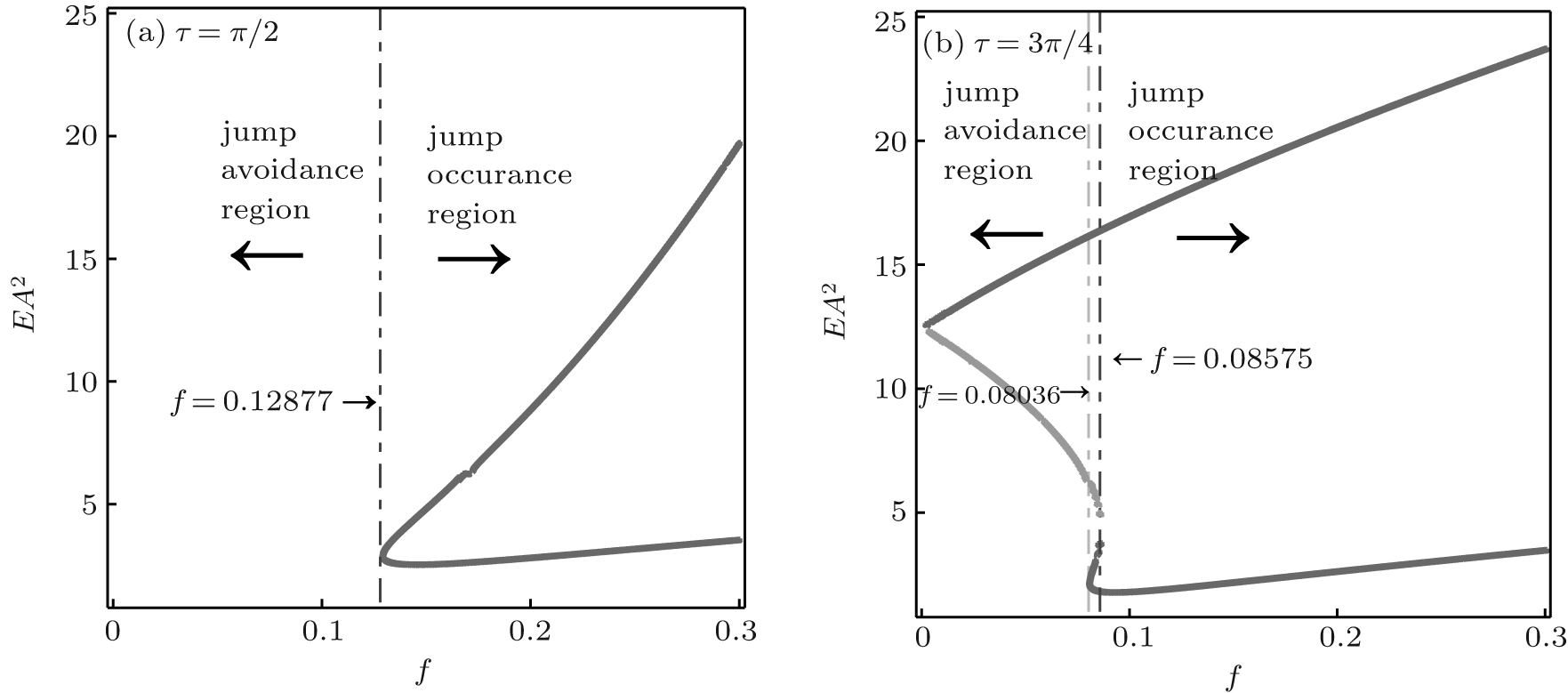 | Fig. 9. No-jump regions indicating the maximum acceptable value of excitation amplitude f for the mean square response. |
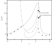
Without loss of generality, when the excitation amplitude and frequency are given as f = 0.2 and Ω = 1.05, figure 10 shows the variations of mean square response EA2 when time delay is taken as a control parameter. The solid line represents the mean square response curve derived from Eq. (25). In addition, according to inequality (24), we also obtain the stability boundary of the mean square response, which has the same shape as that for the deterministic case.
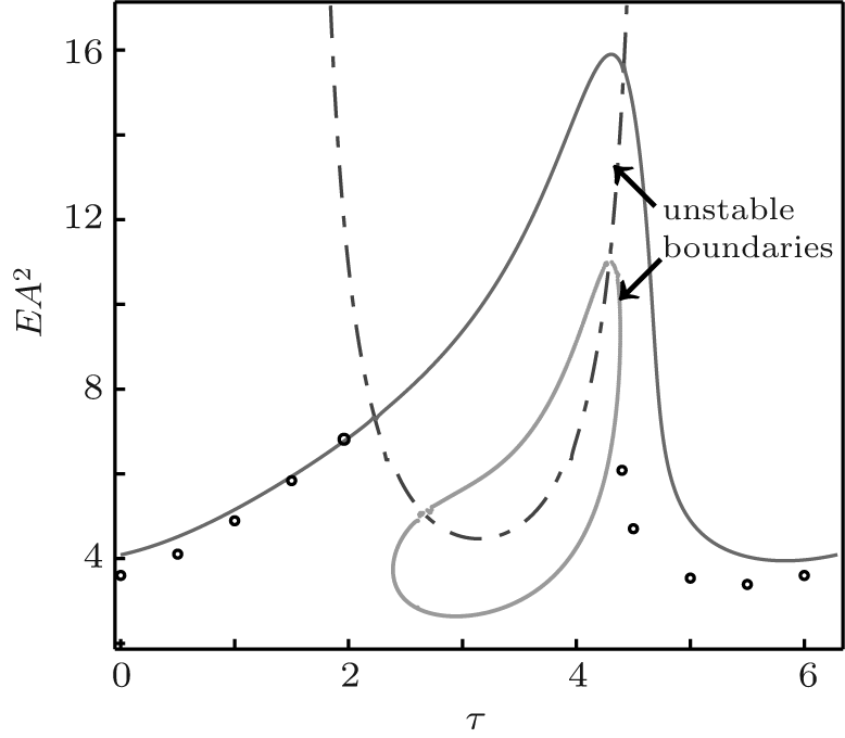 | Fig. 10. Mean square responses versus time delay (solid line: mean square response curve). |
Finally, in order to study the effect of noise intensity on the response of system (2) more clearly, phase portraits and response time histories of system (2) are plotted in Fig. 11. The parameters of system (2) are just the same as those in the previous section, while time delay τ = π /2 is given as an example. Compared with the case in Figs. 11(d), 11(e), and 11(f), the random noise γ W(t) may change the response of system (2) from a periodic solution to a quasiperiodic one, and the corresponding phase trajectory can be changed from a limit cycle to a diffused limit cycle. Further numerical simulation shows that the width of the diffused limit cycle increases with the increase of the noise intensity. However, the topological property of the system does not change.
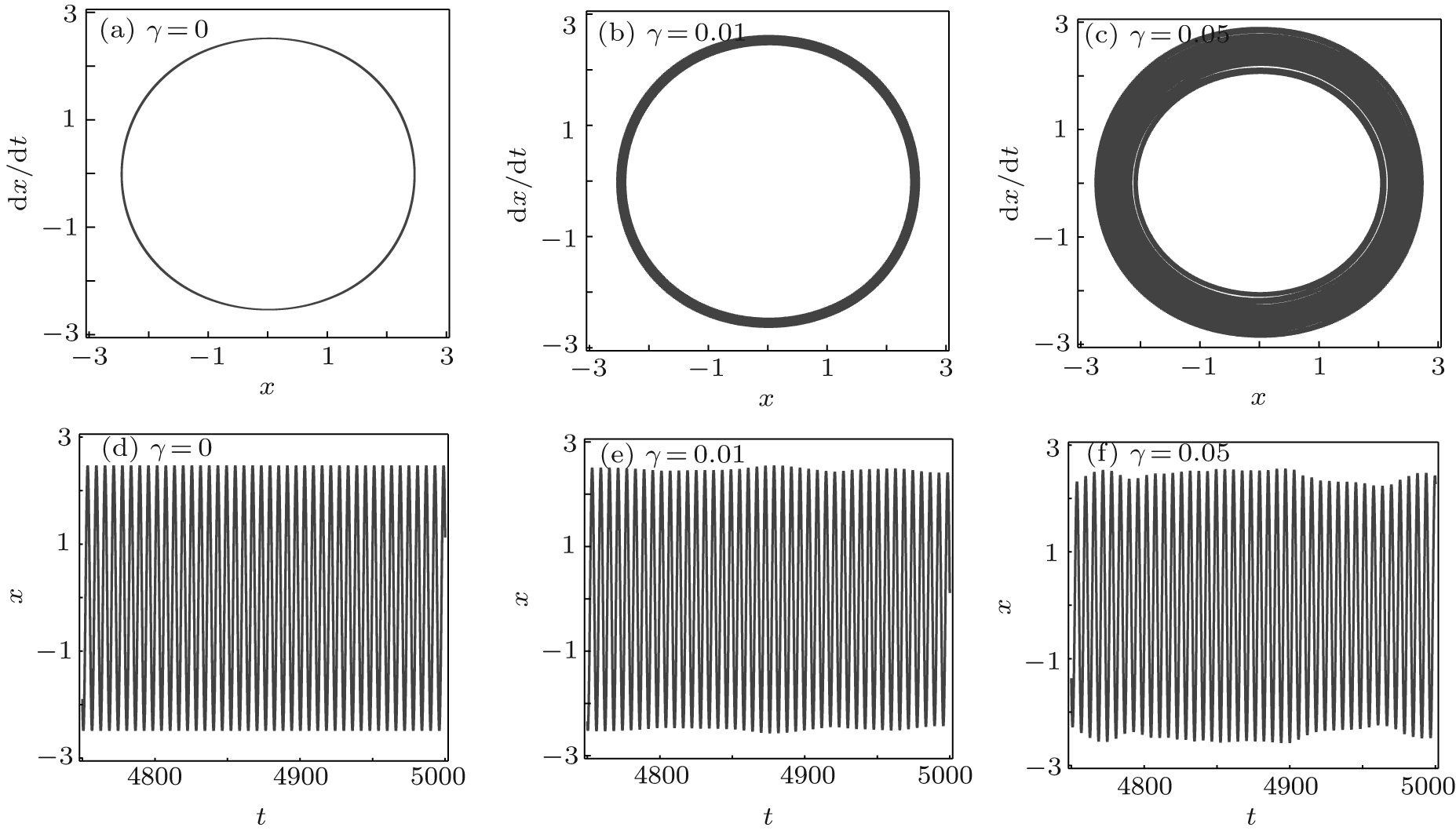 | Fig. 11. Phase portraits and time histories with time delay τ = π /2. |
In the present paper, the principal resonance responses of an EI system with cubic time-delayed velocity feedback and narrow-band random excitation are studied. Multi-valued responses are found, in contrast to the traditional frequency response curve, [32] where the middle of the three solutions is unstable, and the smallest and largest ones are stable, only the smallest amplitude of the response is stable under certain time delays, which is also demonstrated by numerical integration and found in Ref. [33] as well. Then, the jump avoidance condition is obtained. For the case without random disturbance, the effects of feedback parameters on the steady-state response as well as the size, shape, and location of stability regions are discussed. Meanwhile, the classification of steady-state solutions is also discussed. For the case with small noise intensity, mean square responses display similar characteristics to those for the deterministic case; actually, this is determined by the topological property, which does not change under small noise intensity.
| 1 |
|
| 2 |
|
| 3 |
|
| 4 |
|
| 5 |
|
| 6 |
|
| 7 |
|
| 8 |
|
| 9 |
|
| 10 |
|
| 11 |
|
| 12 |
|
| 13 |
|
| 14 |
|
| 15 |
|
| 16 |
|
| 17 |
|
| 18 |
|
| 19 |
|
| 20 |
|
| 21 |
|
| 22 |
|
| 23 |
|
| 24 |
|
| 25 |
|
| 26 |
|
| 27 |
|
| 28 |
|
| 29 |
|
| 30 |
|
| 31 |
|
| 32 |
|
| 33 |
|