Atomic cooling technology has provided a new stage on which to study ultracold atomic gases. The Bose gases, ^{[1– 4]} Fermi gases, ^{[5– 7]} and boson– fermion mixtures^{[8– 11]} have been studied both experimentally and theoretically. In recent years, superfluid Fermi gases have attracted much attention, and the superfluidity of ultracold fermions in optical lattices has been established.^[12] Many phenomena and questions have also been studied, such as superfluid-insulator transition, ^{[13, 14]} collective excitations, ^{[15, 16]} Bloch oscillations, ^{[17, 18]} Josephson oscillations, thermodynamic properties, ^{[19, 20]} pseudogap phenomenon, ^[21] quantized superfluid vortex rings, ^[22] Landau– Zener tunneling, and Rosen– Zener tunneling.^{[23– 26]}

As we know, the crossover from a BEC regime to a unitarity regime has been an intense area of research via the Feshbach resonance technique. This allows one to change the system from the BEC to the unitarity regime by changing the s-wave scattering length α _f. When α _f → + 0, the system is in a BEC regime, when α _f → + ∞ , the system is in a unitarity regime. In general, the scattering length α _f is an adjustable parameter and plays an important role in the dynamics of Fermi superfluid gases.

However, up to now, it is not clear that the scattering length and other system parameters influence the trapping and tunneling of the superfluid Fermi gases in an accelerating optical lattice. We try to study how the scattering length and other system parameters influence the trapping and tunneling, which would offer a good understanding in an accelerating optical lattice. So, in the present paper, we study the tunneling dynamics of Fermi gases both analytically and numerically in optical lattices. It is shown that there are four different phases, which are Josephson oscillation (JO), oscillating-phase-type self-trapping (OPTST), running-phase-type self-trapping (RPTST), and self-trapping (ST).^{[27– 33]} It is noted that the number density of the Fermi gas and the scattering length play a crucial role on the the trapping and tunneling of the Fermi gases. Some phenomena are observed and the explanations are given. In some regimes, all transfer can be obtained. On the contrary, in the other regimes, the quantum transition can be completely blocked.

The article is organized as follows. In Section 2, the models are presented. In Section 3, we discuss the energy and the scattering length of different cases in the BEC regime, and obtain the critical scattering length and critical Hamiltonian. The relationship between the critical scattering length, the number density n₀, and the coupling coefficient v are analyzed. In Section 4, the tunneling phenomena of superfluid Fermi gas in the BEC regime are observed. In Section 5, we give the theoretical explanation of tunneling phenomena. In Section 6, the conclusion is presented.

We consider condensed rotating superfluid Fermi gases in the one-dimensional accelerating optical lattices. For large numbers of Na atoms, we assume that the Cooper pair size is smaller than the lattice spacing. At sufficiently low temperatures, the dynamical behavior of superfluid Fermi gases can be modeled by the one-dimensional nonlinear Schrö dinger equation^[34]

where M = 2m, and m is the mass of one atom. k_L is the wave number of the laser light, and we apply an optical lattice with a wave number of k_L = 2π /λ , where λ = 1064 nm is the wavelength of the laser beam used to derive the lattices. v₀ is the depth of the lattice potential. A force of Ma_l is represented in the vector potential gauge, which may stand for either the inertial force in the co-moving frame of an accelerating lattice or the gravity force. μ is the chemical potential of the superfluid Fermi gases. ϕ is the wave function. After the following change of variables,

where n₀ is the average particle density, we can obtain a dimensionless form of Eq. (1) as follows:

The μ can be given as follows:^{[35, 36]}

where

we provide that , and v = 1.1, η = 22.22, which will make the bulk chemical potential Eq. (4) satisfy the correct unitarity limit μ (n, α _f) = 22.22ħ ²n^2/3/m.^{[37, 38]} So equations (4) and (5) can be made to satisfy the correct weak-coupling and unitarity limit. Parameters α and γ are constants, and v represents the smooth interpolation of f(x) between small and large x values.^[36] We give , ñ = n/n₀ and then we can obtain a dimensionless chemical potential:

In the small-gas-parameter (x → + 0) regime, or in the BEC regime, equation (5) becomes

In this case, μ can be approximated by retaining from the first to the sixth lowest terms in the small-gas-parameter regime as follows:

where c₁ = α _fn₀/2k_L, , and , , .

In the case of x → + ∞ , or in the unitarity regime, equation (5) becomes

and

where , , and .

At the first Brillouin zone edge, the wave function can be written as ϕ = ae^ix/2 + be^{− ix}/2 (a and b are the probability amplitudes of atoms in each of the optical lattice, | a| ² + | b| ² = 1). We obtain the following equations from Eq. (3)

where d₁ = c₁ + c₂ + c₃ + c₄ + c₅ + c₆, d₂ = c₁ + 3c₂/2 + 11c₃/6 + 2c₄ + 7c₅/3 + 5c₆/2, d₃ = 3c₂/4 + 55c₃/36 + 2c₄ + 28c₅/9 + 15c₆/4, and d₄ = − 3c₂/16– 55c₃/432 + 14c₅/27 + 15c₆/16 are in the BEC regime, and d₁ = c₁ + c₂ + c₃ + c₄, d₂ = 2c₁/3 + c₂/3− c₃/6, d₃ = − 2c₁/9− 2c₂/9 + 7c₃/36, and d₄ = 4c₁/27 + 5c₂/27– 91c₃/432 are in the unitarity regime.

Setting a = | a| e^{iθ _a}, b = | b| e^{iθ _b}, defining the population difference s = | b| ² – | a| ² and the relative phase θ = θ _b – θ _a, we obtain

where δ = − α t is the energy bias, and d₂, d₄ are the nonlinear parameters describing the interaction. Equations (13) and (14) can be cast into the canonical form: ds/dt = − ∂ H/∂ θ , dθ /dt = ∂ H/∂ s with the classical Hamiltonian defined as

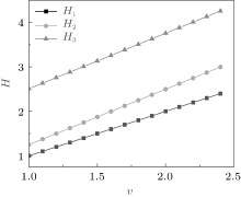
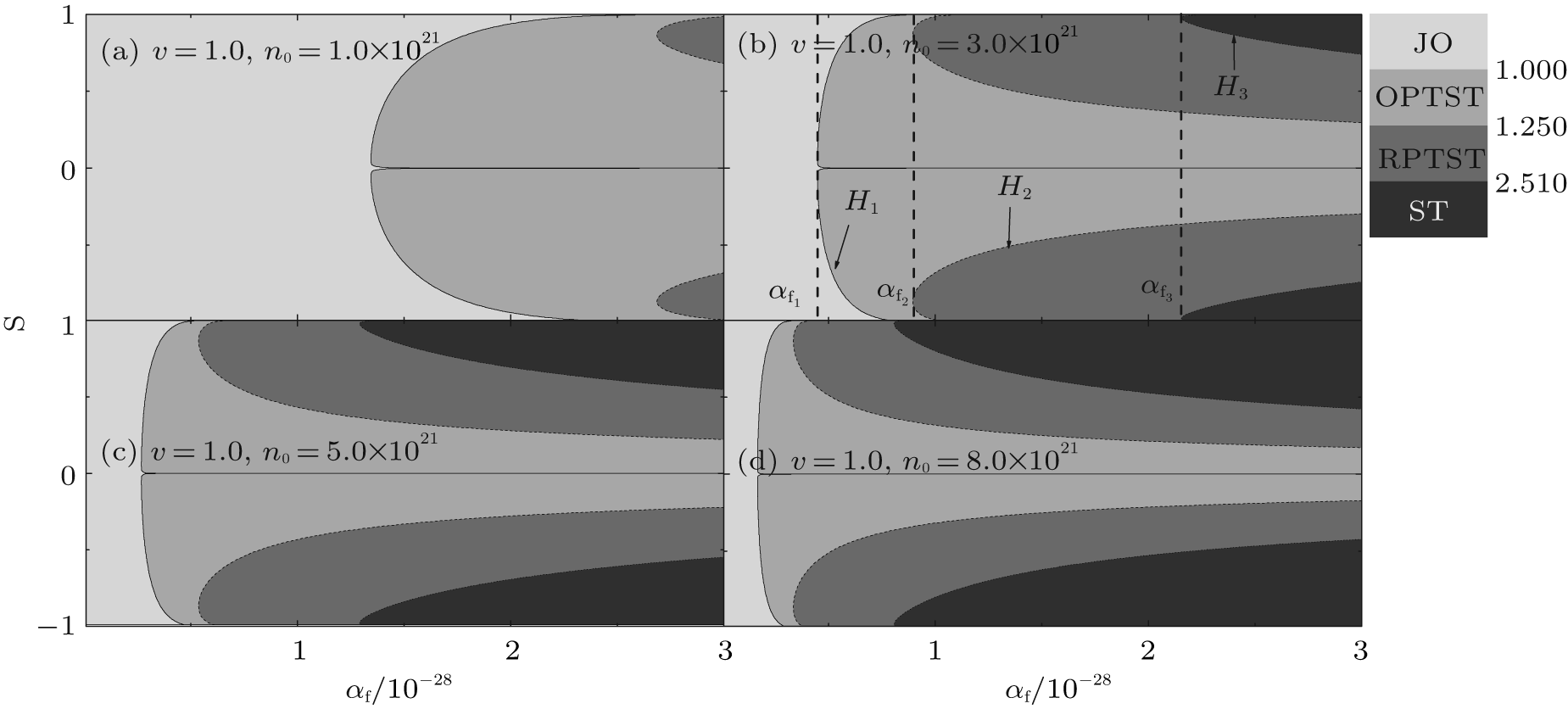
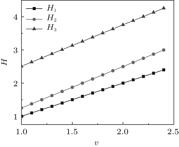
Now we consider the system which is in the BEC regime where we set δ = 0, and exploit the 4– 5th Runge– Kutta algorithm to numerically solve Eq. (13) and (14). The dependence of the system energy H on the scattering length α _f, the number density n₀ and the population difference s are shown in Fig. 1. It indicates from Fig. 1 that the system energy depends on the population difference, the scattering length, and the number density. It is also noted from Fig. 1 that there are four phases of JO, OPTST, RPTST, and ST. The boundary curves between JO and OPTST, OPTST and RPTST, and RPTST and ST are represented by H₁, H₂, and H₃ respectively. The corresponding critical scattering lengths are α _f1, α _f2, and α _f3. It is noted that the critical energies of H₁, H₂, and H₃ depend on the system parameter v. The relationships between parameter v and the critical energies are given in Fig. 2.

Fig. 1.

	Figure Option ViewDownloadNew Window
	Fig. 1. Dependence of H on the system parameter α f and n0 in the BEC regime, where θ = π , v = 1.0.

Fig. 2.

	Figure Option ViewDownloadNew Window
	Fig. 2. Dependence of H1, H2, and H3 on the parameter v in the BEC regime, where n0 = 3.0 × 1021.

Equation (13) can be rewritten as follows: if δ = 0 and θ = π

The critical energies can be obtained as follows:

obviously, d₂ and d₄ are the function of α _f and n₀. That is to say d₂₁ = d₂(α _f1, n₀), d₄₁ = d₄(α _f1, n₀), d₂₂ = d₂(α _f2, n₀), d₄₂ = d₄(α _f2, n₀), d₂₃ = d₂(α _f3, n₀), and d₄₃ = d₄(α _f3, n₀). Dependence of the critical scattering lengths α _f1, α _f2, and α _f3 on the system parameters of v and n₀ are given in Fig. 3.

Fig. 3.

	Figure Option ViewDownloadNew Window
	Fig. 3. Dependence of α f1, α f2, and α f3 on the parameter v in the BEC regime.

We find that similar phenomena will appear in the Bosen system; the different phases (OPTST, RPTST, and ST) are found by adjusting the system parameters.^{[23, 24, 39]} However, in the paper, our work is different from the Boson systems. We find critical scattering lengths of different phases, which would provide a good way of self-trapping for the Fermion system in the experiment.

As is well known, the scattering length α _f can be adjusted in the experiment by the Feshbach resonance technique; for this reason, we study the phase transition by adjusting the scattering length α _f. We assume that the scattering length α _f changes with time t as follows:

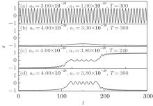
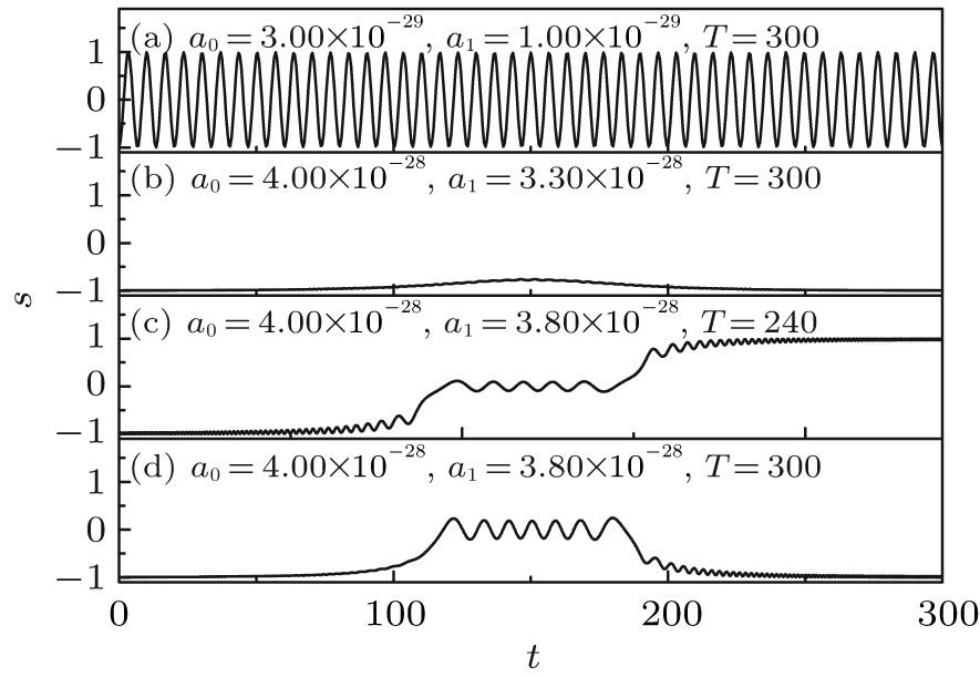
where a₀, a₁, and T are adjustable parameters. a₁ = 0 in the regions of both t ≤ 0 and t ≥ T. Setting the initial conditions of the number density n₀ = 3.0 × 10²¹, ^[34]v = 1.0, and s ≈ − 1, solving Eq. (13) and Eq. (14), we obtain the numerical results which are presented in Fig. 4.

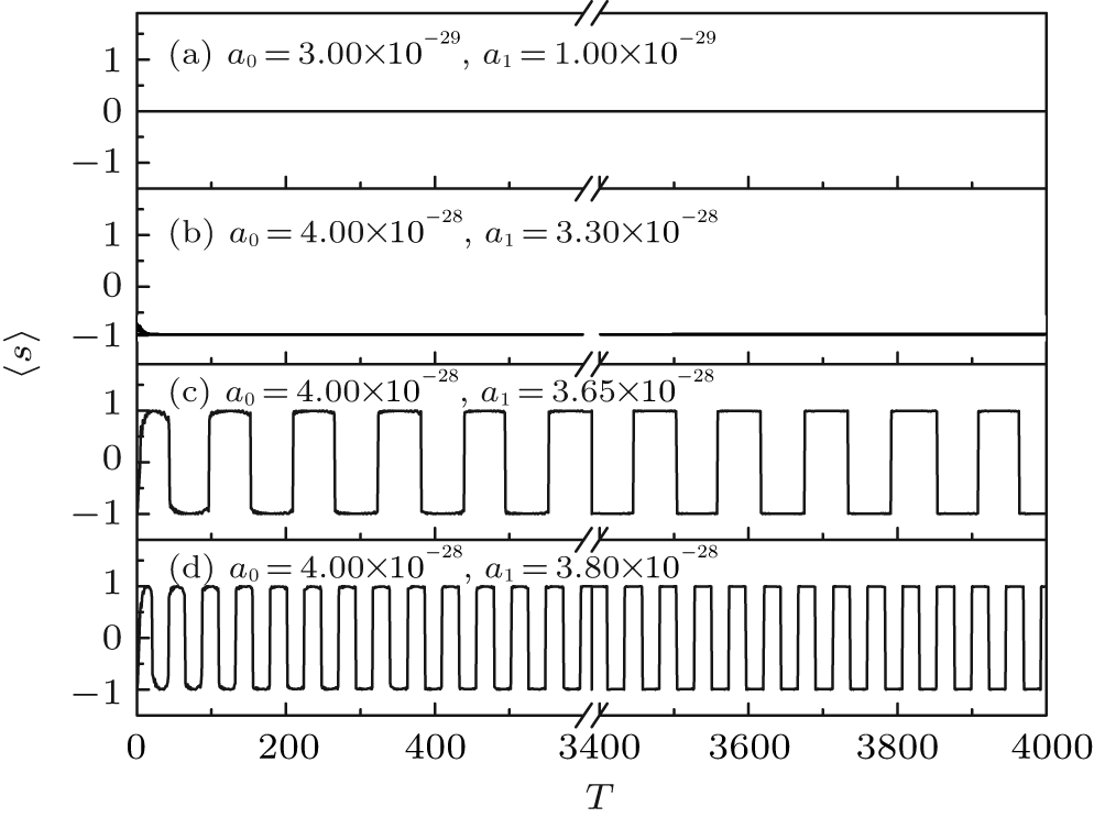
First, we choose the system parameters as follows: T = 300, (a₀, a₁) = (3.00 × 10^{− 29}, 1.00 × 10^{− 29}), and the results are shown in Fig. 4(a). Second, T = 300, (a₀, a₁) = (4.00 × 10^{− 28}, 3.30 × 10^{− 28}), and the results are shown in Fig. 4(b). Third, we choose (a₀, a₁) = (4.00 × 10^{− 28}, 3.80 × 10^{− 28}) but with different values of T, and the results are shown in Fig. 4(c) and Fig. 4(d). It is noted from the results that the transition probability s ≈ − 1 or s ≈ 1 depends on the system parameters T, a₀, and a₁. In order to understand how the system parameters affect the transition probability, the dependence of the transition probability on the system parameters is presented in Fig. 5.

Fig. 4.

	Figure Option ViewDownloadNew Window
	Fig. 4. Profile of population difference versus time t for different system parameters (a) T = 300, (a0, a1) = (3.00 × 10− 29, 1.00 × 10− 29), (b) T = 300, (a0, a1) = (4.00× 10− 28, 3.30 × 10− 28), (c) T = 240, (a0, a1) = (4.00 × 10− 28, 3.80 × 10− 28), (d) T = 300, (a0, a1) = (4.00 × 10− 28, 3.80 × 10− 28).

Fig. 5.

	Figure Option ViewDownloadNew Window
	Fig. 5. Dependence of transition probability on the system parameter T for different values of a0 and a1, (a) (a0, a1) = (3.00 × 10, 1.00× 10− 29), (b) (a0, a1) = (4.00 × 10− 29, 3.30 × 10− 28), (c) (a0, a1) = (4.00 × 10− 28, 3.65 × 10− 28), (d) (a0, a1) = (4.00 × 10− 28, 3.80 × 10− 28).

It is observed from Fig. 5(a) that there are no self-trapping phenomena in which the system parameters are (a₀, a₁) = (3.00 × 10^{− 29}, 1.00 × 10^{− 29}). However, figure 5(b) shows that the self-trapping phenomena happen where the system parameters are (a₀, a₁) = (4.00 × 10^{− 28}, 3.30 × 10^{− 28}). Interesting phenomena are observed in Fig. 5(c) and in Fig. 5(d) where the system parameters are (a₀, a₁) = (4.00 × 10^{− 28}, 3.65 × 10^{− 28}) and (a₀, a₁) = (4.00 × 10^{− 28}, 3.80 × 10^{− 28}) respectively. It is noted that the transition probabilities change with T periodically and a rectangular periodic pattern emerges. The periodicity of the rectangular wave increases with a decrease of the parameter a₁, which is similar to that found previously.^[40]

Most articles study tunneling by changing the coupling strength between two modes to adjust the particle distribution between the two modes in the Bosen system.^{[25, 41, 42]} The periodicity of the rectangular wave of a fermion system is similar to the Boson system, but the regular periodicity is different from the Boson system.

The classical Hamiltonian determines the adiabatic evolution of quantum eigenstates corresponding to the movement of fixed points.^[41] In order to obtain the fixed points, we set ds/dt = 0 and dθ /dt = 0 in Eq. (13) and Eq. (14) and then we obtain

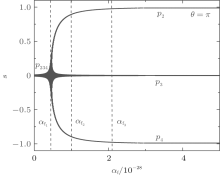
where the signs of ± correspond to θ = 0 and θ = π respectively. For the case of δ = 0, we can obtain two fixed points: (s_f, θ _f) = (0, 0) and (s_f, θ _f) = (0, π ). The numerical results of Eq. (21) are presented in Fig. 6 for the BEC regime.

Fig. 6.

	Figure Option ViewDownloadNew Window
	Fig. 6. The fixed points for different values of α f in the BEC regime, where v = 1.0 and n0 = 3.0 × 1021.

It is noted that there is only one fixed point s_f = 0, i.e., in JO when α _f < α _f1, while there are three different fixed points in the region of α _f1 < α _f < α _f3. It seems that the system is in OPTST when α _f1 < α _f < α _f2 and in the RPTST when α _f2 < α _f < α _f3. However, the system is in ST when α _f > α _f3.

We now pay our attention to how the fixed points change as the time t increases from t = 0 to t = T in the adiabatic condition, i.e., T is large enough. It is noted that the fixed points p₂ or p₄ will merge into a new stable fixed point p₂₃₄ when the scattering length changes from initial value α _f = a₀ to α _f = α _f1 (t = t* ). As the time continues to increase, the scattering length changes from α _f = α _f1 to α _f = a₀ − a₁, then from α _f = a₀ − a₁ to α _f = α _f1 (t = T – t* ), and finally to α _f = a₀ (t = T).

As the scattering length changes with time t, an interesting question is at which point will the state choose to follow when p₂₃₄ bifurcates into p₂, p₃, and p₄ at the point of t = T – t* (α _f = α _f1). Since p₃ is an unstable fixed point, we will not consider it.

The state that follows p₂ will give a zero value of the adiabatic transition probability (s = 1), whereas the state that follows the p₄ will correspond to a complete population transfer (s = − 1). This classical picture could explain why we see a rectangular pattern in Fig. 5(c) and Fig. 5(d).

In order to explain the phenomena, we need to calculate the instantaneous frequency that characterizes the oscillations around the fixed points. We start from the differential equations (13) and (14), and introduce infinitesimal variables s′ and θ ′ with s = s_f + s′ , and θ = θ _f + θ ′ , where (s_f, θ _f) denote the fixed points. Inserting these expansions into Eq. (13) and Eq. (14), we obtain

Setting (s_f, θ _f) = (0, π ), we obtain the small amplitude oscillation frequencies

the critical point can be given as follows:

Based on the above analyses, we also know that t^* should conform to the above equation, and the algebraic expression of t′ is given. The relationship between t^* , t′ , and parameter a₀ is also presented in Fig. 7,

Integrating ω (t) from t^* to t′

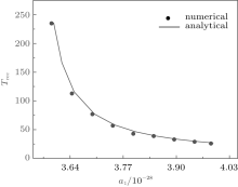
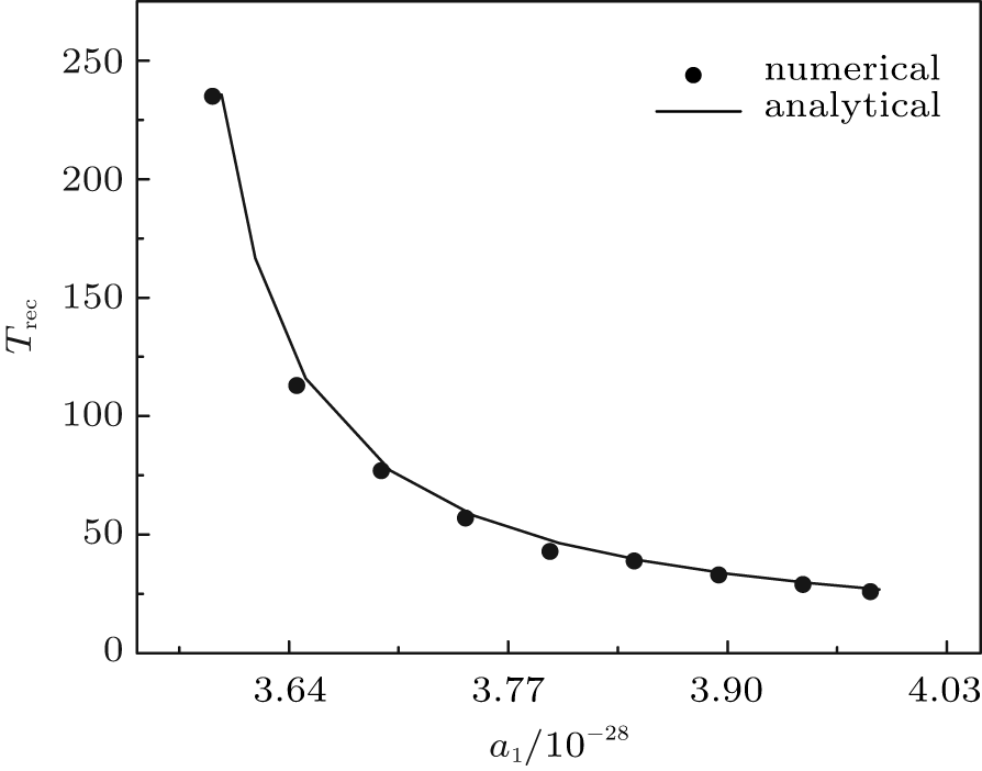
thus the period of rectangular oscillation observed in Fig. 6 under adiabatic limit can be expressed as

Fig. 7.

	Figure Option ViewDownloadNew Window
	Fig. 7. Dependence of the t* and t′ on the system parameter a1, where v = 1.0 and a0 = 4.00 × 10− 28.

The numerical results from Eq. (13) and Eq. (14) are compared with the analytical results from Eq. (28) and a good agreement is observed in Fig. 8.

Fig. 8.

	Figure Option ViewDownloadNew Window
	Fig. 8. Period of rectangular oscillation versus the parameter a1 under the adiabatic limit, where v = 1.0 and a0 = 4.00 × 10− 28.

In this paper, we studied the tunneling dynamics of the Fermi gas in an optical lattice in the BEC regime. Four different cases of JO, OPTST, RPTST, and ST are presented. It is noted that the s-wave scattering length plays a crucial role on the tunneling dynamics. The three critical scattering lengths and the four regions of the system energies are also found. By adjusting the scattering length in the adiabatic condition, we find that the transition probabilities change with the adiabatic periodicity and a rectangular periodic pattern emerges. The periodicity of the rectangular wave depends on the system parameters such as the periodicity of the adjustable parameter, the s-wave scattering length. So the Fermi superfluid gases can be controlled about the tunneling phenomenon and the macroscopic quantum properties. Finally, the numerical results and analytical results further show a good agreement.