

Spatial snowdrift game in heterogeneous agent systems with co-evolutionary strategies and updating rules*
[Xia Hai-Jiang, Li Ping-Ping, Ke Jian-Hong† , Lin Zhen-Quan]
, Lin Zhen-Quan]
|
|


†Corresponding author. E-mail: kejianhong@ymail.com
*Project supported by the National Natural Science Foundation of China (Grant Nos. 11175131 and 10875086).
We propose an evolutionary snowdrift game model for heterogeneous systems with two types of agents, in which the inner-directed agents adopt the memory-based updating rule while the copycat-like ones take the unconditional imitation rule; moreover, each agent can change his type to adopt another updating rule once the number he sequentially loses the game at is beyond his upper limit of tolerance. The cooperative behaviors of such heterogeneous systems are then investigated by Monte Carlo simulations. The numerical results show the equilibrium cooperation frequency and composition as functions of the cost-to-benefit ratio r are both of plateau structures with discontinuous steplike jumps, and the number of plateaux varies non-monotonically with the upper limit of tolerance νT as well as the initial composition of agents f a0. Besides, the quantities of the cooperation frequency and composition are dependent crucially on the system parameters including νT, f a0, and r. One intriguing observation is that when the upper limit of tolerance is small, the cooperation frequency will be abnormally enhanced with the increase of the cost-to-benefit ratio in the range of 0 < r < 1/4. We then probe into the relative cooperation frequencies of either type of agents, which are also of plateau structures dependent on the system parameters. Our results may be helpful to understand the cooperative behaviors of heterogenous agent systems.
The widespread phenomenon that cooperation emerges spontaneously in competitive groups consisting of selfish individuals has drawn much attention.[1– 6] To understand such a phenomenon, scientists have taken advantage of game models to study the cooperative behaviors in competitive systems, and they have made great progress.[7– 11] Especially, the prisoner’ s dilemma game (PD)[12] and the snowdrift game (SG)[13, 14] have been employed and investigated widely in the literature. In these game models, two agents can choose to either cooperate (C-strategy) or defect (D-strategy) in their interactions. Each agent can get a payoff R if they both use the C-strategy and a payoff P if they both use D-strategy. If one chooses the C-strategy while another picks up D-strategy, the defector will receive the highest payoff T while the cooperator only gains the sucker’ s payoff S. The PD has the payoff ordering of T > R > P > S and 2R > (T + S), while the SG differs from the PD only in the payoff ordering, namely, it is characterized with T > R > S > P.
Recently, considerable research works have been devoted to investigating the emerging and promoting of cooperation in the evolutionary PD or SG.[15– 23] One key spirit of evolutionary games is that each agent need not persist in a sole strategy forever and can adapt it according to a certain updating rule. A variety of updating rules have been introduced in the literature, [15, 24– 33] which can be classified into two distinct categories. One is the class of imitation-type updating rules, such as the Fermi rule, [24] the replicator rule, [26, 27] and the unconditional imitation rule.[15, 29] For example, when an agent adopts the unconditional imitation rule, he always imitates the strategy of the agent with the highest payoff among his neighbors and himself. Imitation-type rules differ from one another only in the object and probability of imitation. Another is the class of self-directed rules, which depends on agents’ own past experience. For instance, Wang et al. proposed a memory-based updating rule, [30] in which each agent records his own successful strategies in previous m rounds and then updates his strategy in the next round according to this pool of strategies. It is very sound to introduce the character of memory in many dynamical processes.[34– 38]
It should also be pointed out that most of the research works only paid attention to the PD and SG in homogeneous agent systems, namely, all the agents obeying the same updating rule (see, e.g., Refs. [13], [30], [39]– [41] and references therein). However, for many real-world systems, the heterogeneity of agents is worthy of serious consideration. To the best of our knowledge, only a few papers are devoted to game dynamics in heterogenous systems, in which agents might adopt the same updating rule but with different parameters[42] or different imitation-type rules.[43– 45] In our previous work, [46] we consider that different agents are of quite a distinct nature and thus divide the agents into two distinct types: copycat-like and inner-directed. Copycat-like agents are neighbor-dependent and follow one of the above imitation-type updating rules, while inner-directed agents are independent and take the memory-based updating rule. The results showed that the cooperative behaviors in the SG of such a heterogeneous system depend crucially on the composition of the two mixing agents.[46]
Since agents participating in the evolutionary games are intelligent, they might self-question their own updating style and change it after some failure experience. Thus, it might be more practical to consider that agents’ updating rules are not unchangeable in the whole course of evolution. Our previous work was only devoted to the SG system with the updating rule of each agent keeping unchanged throughout the evolution.[46] In this work, we will further probe into the evolution dynamics of the SG in heterogeneous agent systems with co-evolutionary strategies and updating rules. The system consists of copycat-like and inner-directed agents. Copycat-like agents obey the unconditional imitation rule while inner-directed ones choose the memory-based updating rule proposed by Wang et al.[30] Moreover, in the course of evolution, a copycat-like agent could change into an inner-directed one after several successive failures due to adopting the imitation-type updating rule, and similarly, an inner-directed agent would become a copycat-like one if he suffers sequential failures by using the memory-based rule. By numerical simulations we investigate in detail the cooperative behaviors in the evolutionary SG of heterogenous agent systems.
The results show that the cooperation frequency in the heterogenous agent system also exhibits discontinuous plateau structures and the number of plateaux is dependent on the system parameters, as in the systems with a fixed composition of agents.[46] Besides, the equilibrium composition of agents is also of a discontinuous plateau structure. As for the system that the copycat-like agents adopt updating rules other than the unconditional imitation rule, we will defer it to a future work.
This paper is organized as follows. In Section 2, we briefly introduce the snowdrift game in heterogenous systems with co-evolutionary strategies and updating rules. In Section 3, we present the simulation results and then discuss the cooperative behaviors. A summary is given in Section 4.
In this work, we aim to investigate the influence of the agent heterogeneity on the game dynamics. Consider a heterogenous system with two types of distinct agents: A-type and B-type. Agents are located on a two-dimensional (2D) square lattice with periodic boundary conditions, and each pair of neighboring agents plays the evolutionary snowdrift game (ESG). For simplicity, the payoffs in the SG can be represented by the following matrix:[12]

Here, the parameter r denotes the cost-to-benefit ratio of mutual cooperation and 0 < r < 1 in the SG. In a round, the agent uses the same strategy to play the pairwise SG with all of his neighbors and gets the total payoff by summing over all payoffs gained in the interactions with his neighbors. For instance, in one round, an agent adopts the C-strategy to play SGs with his four neighbors, among who there are x agents using the C-strategy and 4 − x agents using D-strategy, then his total payoff is equal to x · 1 + (4 − x) · (1 − r); conversely, if he adopts the D-strategy to play SGs with the same neighbors, then his total payoff is equal to x · (1 + r) + (4 − x) · 0. Next, based on the value of the total payoff, this agent will change his type or update his strategy used in the next round according to a certain rule.
In our system, A-type agents are inner-directed and obey the memory-based rule (MB), [30] while B-type agents are copycat-like ones and take the unconditional imitation rule (UI).[14] The two updating rules are described briefly as follows:[46]
(i) Memory-based rule In each round, besides the actual total payoff obtained in practical interactions between neighbors, the agent also calculates a virtual total payoff by using the anti-strategy to play virtual games with his neighbors. The agent then makes a comparison between the actual and virtual payoffs and labels the strategy with higher payoff as the successful one in this round. In view of the finiteness of human memory, we assume that each agent has a limited memory chain of length m and can only note down the successful strategies in the recent m rounds. In the next round, the agent will count the number of C strategies recorded in his memory chain, say mc, and then adopts the C-strategy with a probability of pC = mc/m (or correspondingly, the D-strategy with a probability of pD = 1 − pC).
(ii) Unconditional imitation rule In the end of each round, the agent analyzes the data of payoffs his neighbors obtained in the current round. If the agent himself has the maximum payoff, then he will continue to use his current strategy in the next round; otherwise, he will pick up the strategy of the neighboring agent(s) with the highest payoff as his next strategy. Moreover, if there is more than one neighbor having the same maximum payoff other than the agent himself, then one of them is selected randomly.
Since in real-world systems agents cannot update their strategies at the same time, we will adopt the asynchronous updating method in this work. In every Monte Carlo step (MCS), agents update their strategies in a random sequence and each agent has a chance to update his strategy on average.[47] Meanwhile, in each round, besides the actual total payoff, each agent also computes out the virtual total payoff by using the anti-strategy to play virtual games. If the virtual total payoff is larger than the actual one, the agent then records this round as a failure (or losing the game). It is sound that agents can accept failure now and then but cannot endure too many sequential failures. On the other hand, agents might not change their updating rule easily due to inertia in mind and behavior. So, each agent has an upper limit of tolerance for the sequential failures, beyond which he will thoroughly dissatisfy his current updating rule and then change it into another one. The value of the upper limit of tolerance characterizes an agent’ s degree of inertia. In this work, for simplicity, all agents are assigned the same upper limit of tolerance ν T (here, ν T is a non-zero positive integer). In the course of evolution, each agent will count the number of his sequential failures; and once this number is beyond ν T, he will change his current updating rule into another one (correspondingly, his type is changed) and the number of his sequential failures resets. That is, a copycat-like agent will evolve into an inner-directed one, and vice versa, once the number of his sequential failures is larger than ν T.
Consider a heterogenous agent system with N agents. The initial percentage concentration of A-type agents is set to be fa0 (0 ≤ fa0 ≤ 1.0), while that of B-type agents is 1 − fa0. Obviously, fa0 = 1.0 represents the homogenous system with pure A-type agents, [30] while fa0 = 0 indicates the pure system only with B-type agents.[41] The number of agents in all numerical simulations is the same, N = L × L = 104. This work aims to investigate the dependence of evolution dynamics on the system parameters fa0, r, and ν T. Besides, it is found that for the ESG in the system with pure A-type agents, the memory length is not the key parameter and has some effect only on the value of the cooperation frequency fc.[30] Thus, the memory size of each A-type agent is set as m = 7. Initially, agents are assigned A-type with a probability fa0 or B-type with a probability 1 − fa0; and moreover, each agent chooses either the C or D strategy completely randomly. Each point in data figures is gained by measuring the mean over the last 1000 MCS after a transient MCS of 104 and then averaging over 20 realizations. Unless stated otherwise, the set of parameters remain unchanged for all numerical simulations.
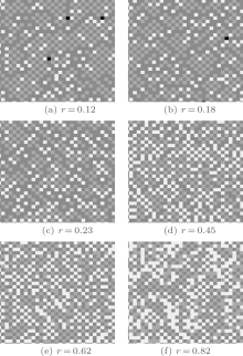
We then perform a series of numerical simulations on a 2D L × L square lattice with periodical boundary conditions. Figure 1 illustrates a set of snapshots gained at MCS = 2 × 10⁴ for different cost-to-benefit ratios, which can show both the strategy distribution and the type composition of agents. By careful statistic analysis of such snapshots one can understand the evolution of cooperation in the heterogenous agent system. In order to characterize the cooperative behavior quantitatively, we define three quantities: the global fraction of cooperators in the total agent of any type fc, the relative fraction of cooperators among A-type agents gca, and the relative fraction of cooperators among B-type agents gcb. Moreover, we define fa as the fraction of A-type agents in the total agent of any type. Obviously, the above-introduced quantities satisfy the relationship fc = fa · gca + (1 − fa) · gcb at any time. At the beginning of the ESG, we have gca = 0.5 and gcb = 0.5. In the following sections, we discuss in detail the cooperative behaviors and the equilibrium composition of agents in heterogeneous agent systems.
 | Fig. 1. Snapshots of spatial patterns of A-type cooperators (blue), B-type cooperators (black), A-type defectors (red), and B-type defectors (yellow) for different cost-to-benefit ratios. (a) r = 0.12; (b) r = 0.18; (c) r = 0.23; (d) r = 0.45; (e) r = 0.62; and (f) r = 0.82. Here, the other model parameters are the same, ν T = 3 and fa0 = 0.5. Obviously, almost all the B-type agents will take the D-strategy eventually and the concentration of A-type agents decreases with the increase of r. |
Since our model has three tunable parameters, we fix the value of the upper limit of tolerance to investigate the dependence of the cooperation frequency (i.e., the fraction of cooperators) and the equilibrium composition on the game parameters.
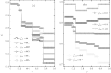
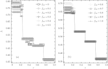
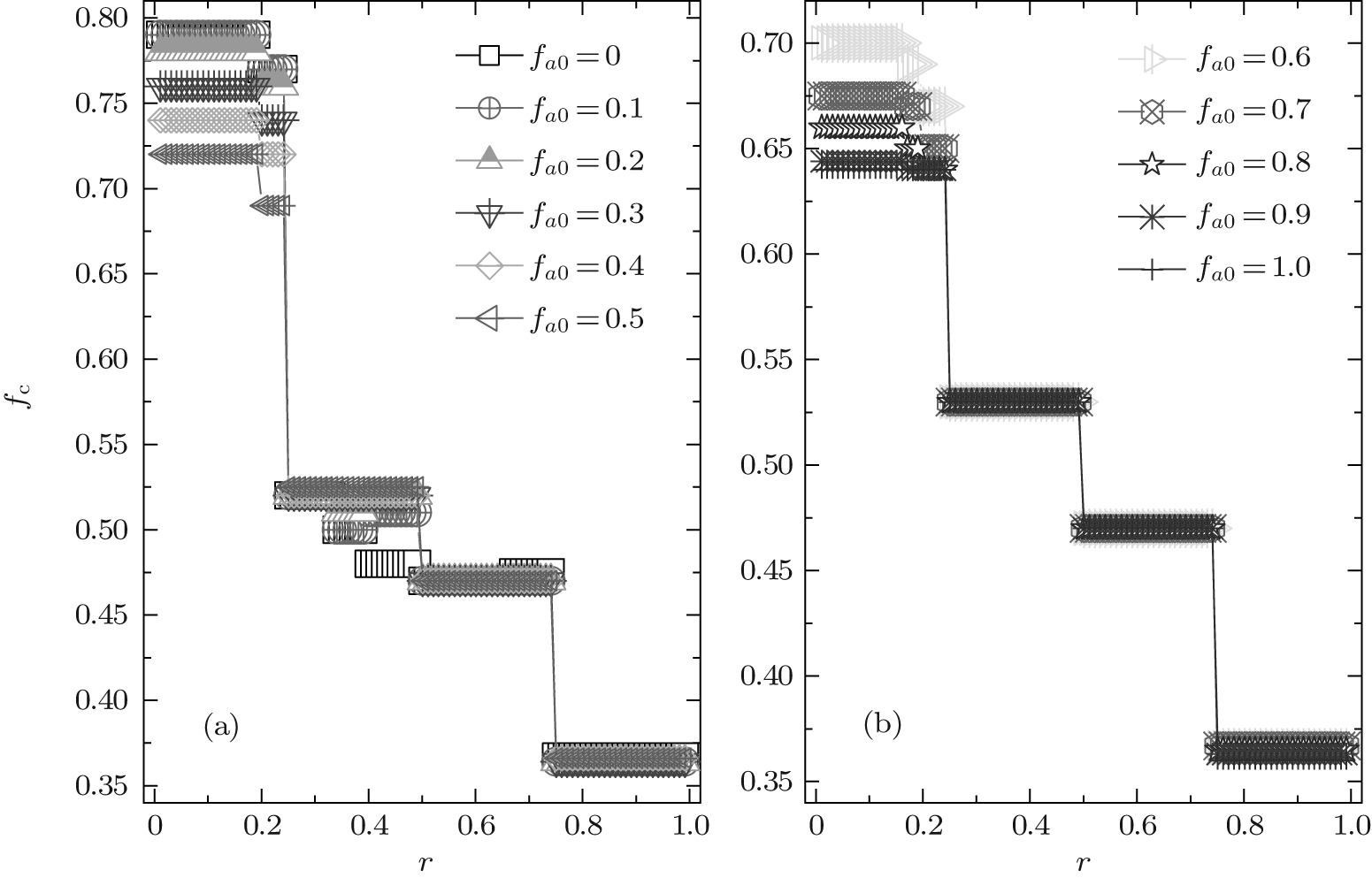
Due to a Chinese proverb, which says “ Not to do anything more than three times” , we first consider ν T = 3. Figure 2 shows a set of the global cooperation frequencies against the cost-to-benefit ratio r for different fa0. Clearly, the global cooperation frequency fc as a function of r is discontinuous and several steplike transitions occur at some particular values of r; moreover, fc is independent of r in each piecewise cooperation level. Thus, fc also has plateau structures in the heterogenous agent systems with co-evolutionary strategies and updating rules, as in the homogenous system with single-type agents[30, 41] as well as the heterogenous system with the fixed composition of agents.[46]
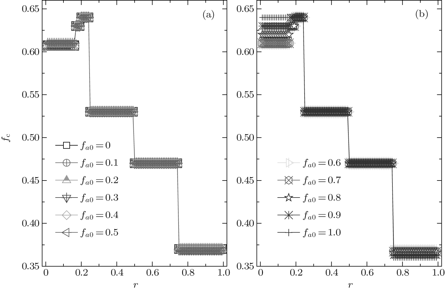 | Fig. 2. The equilibrium cooperation frequency fc as a function of the cost-to-benefit ratio r at ν T = 3. It is shown that fc always exhibits a discontinuous steplike structure for an arbitrary composition fa0, and the value of fc is dependent on fa0 only in the range of 0 < r < 1/4. |
The phenomenon that the global cooperation frequencies are of such steplike structures can be interpreted by analyzing the local stability of configurations.[30, 41] The X-agent surrounded by pC-agents and qD-agents in his neighborhood is denoted by X (pCqD), where X = C (D), p and q are two positive integers. In this work, we investigate the evolutionary snowdrift game on a 2D square lattice, in which each agent will play the pairwise SG only with his four neighbors. Thus, for the configuration X (pCqD), we have the relation p+ q = 4, where p ∈ {0, 1, 2, 3, 4}. Obviously, only ten kinds of possible configurations exist in our system.
Moreover, a C(pCqD)-agent can obtain the total payoff p + q(1 − r), after he plays the SG with his pC-neighbors and qD-neighbors, and similarly, the total payoff that a D(pCqD)-agent gains is equal to p(1 + r). For the system with pure A-type agents, the C(pCqD)-agent will not change into a D(pCqD)-agent only when p + q(1 − r) > p(1 + r), and inversely, the D(pCqD)-agent cannot change into a C(pCqD)-agent if p(1 + r) > p + q(1 − r). So, the balance between the C(pCqD)-agent and D(pCqD)-agent results in the equation p + q(1 − r) = p(1 + r), which yields a series of critical values rc = 1/4, 1/2, and 3/4, as illustrated in Table 1. While, for the system with pure B-type agents, the C(mCnD)-agent (here, m + n = 4) must have the same payoff as his neighboring D(pCqD)-agent so as to keep a local balance, which gives the equation m + (4 − m)(1 − r) = p(1 + r) with the possible solutions listed in Table 2.
| Table 1. The critical transition points in the system with pure A-type agents. |
| Table 2. The critical transition points in the system with pure B-type agents. |
On the other hand, for each pair of configurations listed in Tables 1 and 2, one configuration can prevail over another in a certain range of r while another wins out in the remaining range of r. For instance, the C(3C1D)-agents dominate over the D(3C1D)-agents in the r < 1/4 case while it is just on the contrary in the r > 1/4 case (see Table 1). Thus, after the system evolves to an equilibrium state, only one or several of the ten configurations can survive finally. Since the value of fc of the system is decided by the composition of configurations, the surviving configurations are somewhat different before and after each critical point, which leads to the discontinuity in fc as a function of r and several apparent discontinuous jumps at those critical points. Thus, it can be safely concluded that the emergence of discontinuous jumps is caused by the competition between different configurations. Moreover, when r is in between two neighboring critical points, the dominating configurations are stable and their quantity is thus independent of the value of r, that is, the value of fc will keep constant. So, the global cooperation frequency fc as a function of r is of a discontinuous steplike structure, something like the energy level structure of atoms, due to the fact that our ESG system on the 2D regular lattice only has enumerable configurations and some distinct configurations survive eventually for different intervals of r. From a different perspective, each level of the global cooperation frequency corresponds to a set of configurations by which the system is constituted at the equilibrium state under some corresponding parameters.
In order to make a comparison between the homogenous and heterogenous systems, we recall the results of the pure B-agent system in the small-r case. One can find, by taking the instability of the configurations with D-core (such as D(pCqD)) in small-r cases into further consideration, that the discontinuous transitions in pure B-agent systems cannot emerge at rc < 1/4.[41] For example, the transition point r= 1/5 is caused by the local configuration D(3C1D) coexisting with C(2C2D); but unfortunately, the configuration D(3C1D) cannot survive in the pure B-agent system with r < 1/4 because such a system suppresses the survival of D-agents.[41] However, in the heterogenous agent system with both A-type and B-type agents, the rich-D configuration, such as D(1C3D) and D(2C2D), is possible to form due to the fact that A-type agents can occupy the core of the configurations and prefer the D-strategy in small-r cases.[46] Without any surprise, besides the above-mentioned discontinuous transitions at rc = 1/4, 1/2, and 3/4, we also observe the secondary jumps at rc = 1/6 and 1/5 emerging in the system with co-evolutionary strategies and updating rules, as demonstrated in Fig. 2. As for the critical point rc = 1/7, it is caused by the competition between the two configurations C(0C4D) and D(3C1D); however, the configuration C(0C4D) cannot emerge in small-r cases in which C-agents dominate over D-ones, and thus, the secondary critical transition at rc = 1/7 cannot be observed even in our heterogenous agent system.
Furthermore, as indicated in Fig. 2, the value of the equilibrium cooperation frequency fc is independent of the initial composition of agents in the range of 3/4 > r > 1/5; while, fc slightly decreases with the increase of fa0 if r > 3/4 and it is just on the contrary if r < 1/5. More intriguingly, the piecewise level of fc in the range of 1/6 < r < 1/5 is somewhat higher than that in the range of 0 < r < 1/6 for almost all fa0 except for fa0= 1.0, while the value of the plateau in the range of 1/5 < r < 1/4 is a little higher than that in the range of 1/6 < r < 1/5 for most of fa0 except for fa0 = 0.9 and 1.0. This is an abnormal phenomenon. As we know, based on the scenario that the SG is constructed, agents will be more and more likely to adopt the D-strategy with the increase of r and, thus, the equilibrium cooperation level will decrease with increasing r.
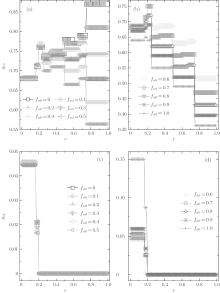
Now we turn to investigate the composition of agents after a long-time evolution. The equilibrium fractions of A-type agents for different fa0 are demonstrated in Fig. 3. It is observed that fa is also of a steplike plateau structure. The value of fa depends crucially on the cost-to-benefit ratio r, and the discontinuous transition points are the same as those for the global cooperation frequency fc. Moreover, the initial value of fa0 also takes an important role in the final composition of agents. For fa0 ≤ 0.8, the equilibrium fraction of A-type agents fa decreases consistently with the increase of r; while for fa0 > 0.8, fa also decreases with increasing r in the range of 0 < r < 1/2, but it is just on the contrary in the range of 1/2 < r < 1. On the other hand, in the range of 1/4 < r < 1, fa always increases consistently with the increase of fa0; while in the remaining range of r, fa is independent of the value of fa0 for fa0 ≤ 0.7 but increases along with fa0 for fa0 > 0.7. Making a comparison between the equilibrium fraction fa and its initial fa0, one can observe that the inequality fa ≥ fa0 is always valid for almost all fa0 except for fa0 = 1.0 and the net difference consistently decreases with increasing fa0 and r. Especially, for fa0 = 1.0 only a little fraction of A-type agents will finally change into B-type ones. Hence, in the ν T = 3 case, A-type agents have fairly little probability of losing three successive games, while it is of high possibility for B-type agents to fail thrice in succession until the fraction of B-type agents decreases to a certain value that depends on the initial parameters fa0 and r.
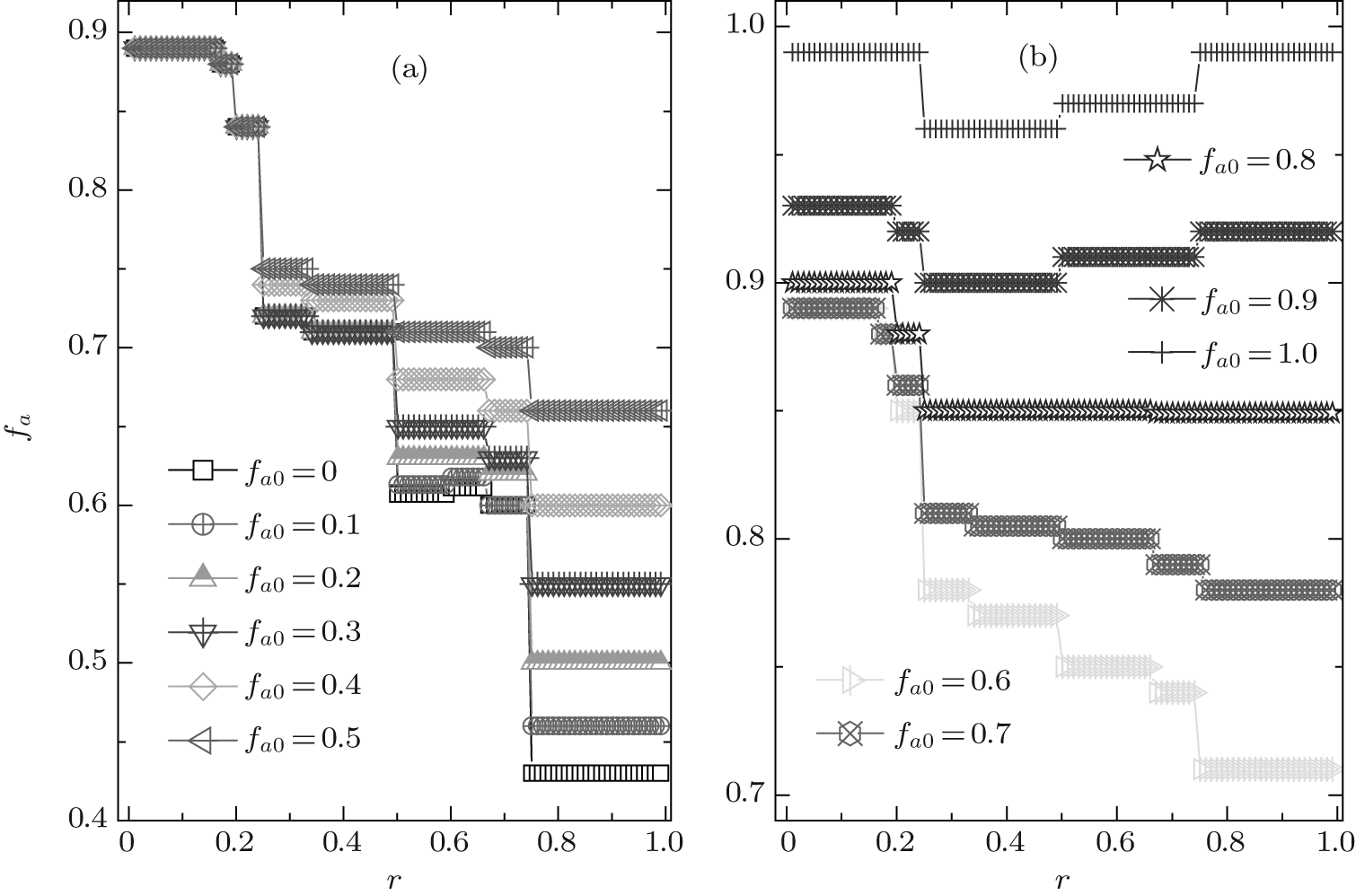 | Fig. 3. The equilibrium composition fa versus the cost-to-benefit ratio r at ν T = 3. It is shown that fa always exhibits a discontinuous steplike structure for each initial composition fa0, and the number of plateaux is related with the value of fa0. |
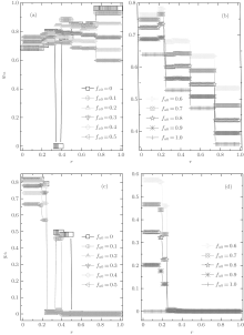
In order to understand the above-mentioned observations, we will probe deeply into the relative cooperative behaviors of both A- and B-type agents at ν T = 3. Figure 4 shows the data lines of the relative cooperation frequencies gca and gcb against r for different fa0. We again find that both gca and gcb as the function of r are of plateau structures. For gcb, there are only three plateaux; while for gca, the number of plateaux is eight when fa0 ≤ 0.7, and with fa0 increasing from 0.7 to 1.0 the number of plateaux decreases to six due to the fact that the discontinuous transitions at rc = 0.4 and rc = 2/3 cannot happen. Moreover, gca is almost independent of the value of fa0 in the range of 0 < r < 1/4 and fa0 ≤ 0.7; while it decays with the increase of fa0 in the remaining range. It is worth noting that for small fa0 the relative cooperation frequency gca is fairly high (for instance, gca > 0.65 for fa0 ≤ 0.3), i.e., most A-type agents adopt the C-strategy. More interestingly, the values of the three levels of gca in the range of 0 < r < 1/4 anomalously enhance with the increase of r, which are in accord with those of the global cooperation frequency fc. As for gcb, it is identically equal to zero in the range of r > 0.2, i.e., all B-type agents adopt the D-strategy independent of the values of fa0 and r, while in the remaining range of 0 < r < 0.2, very few of the B-type agents may take the C-strategy (here, the maximum value of gcb is 0.15 at fa0 = 1.0) and the value of gcb slightly increases with increasing fa0.
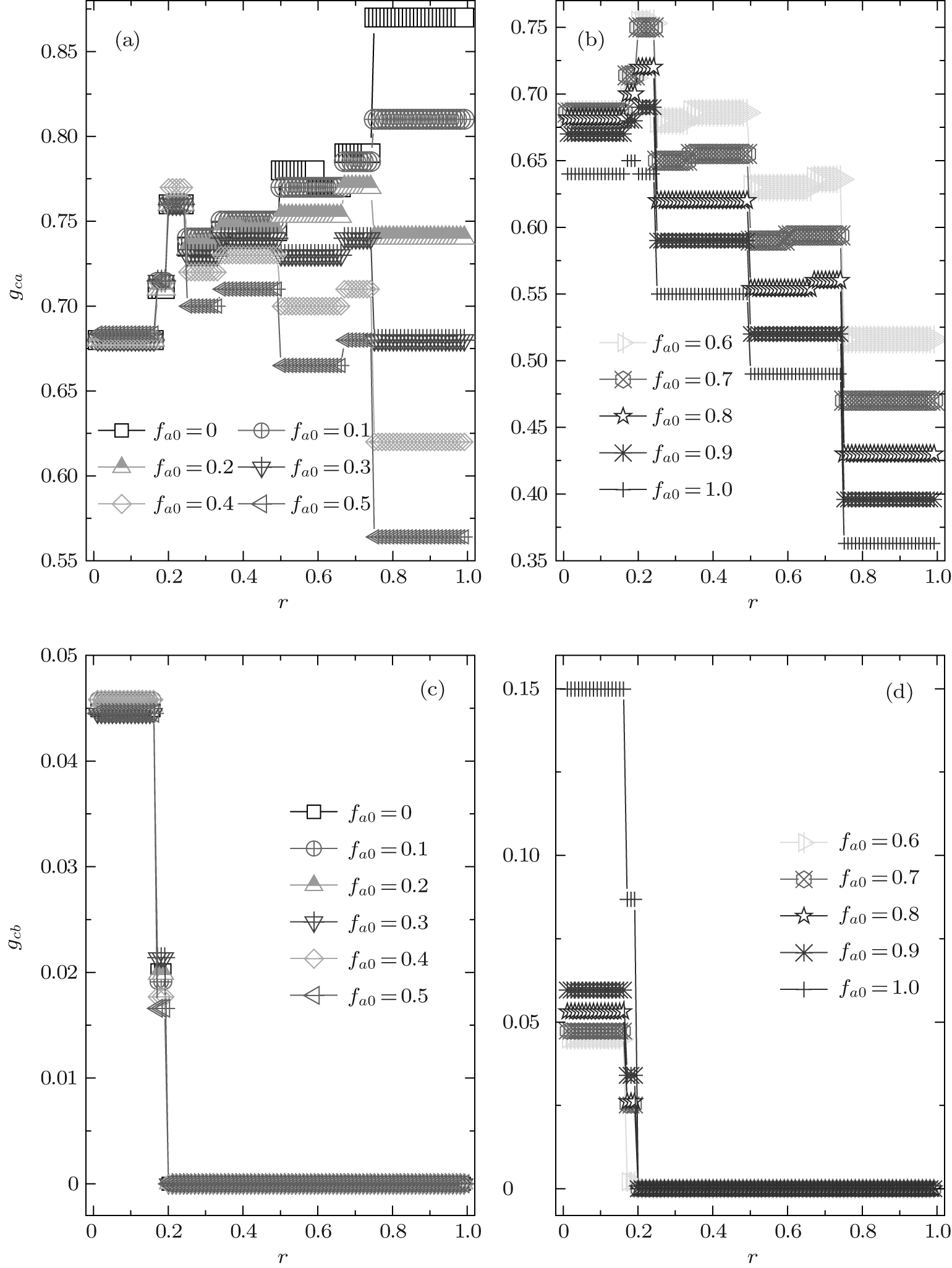 | Fig. 4. The relative cooperation frequencies gca and gcb versus the cost-to-benefit ratio r at ν T = 3. It is shown that both gca and gcb have a discontinuous steplike structure for each initial composition fa0. gca decreases with increasing fa0 while gcb increases with fa0. And gca always has a non-zero value for arbitrary r and fa0, while gcb consistently equals zero in the range of 1/5 < r < 1. |
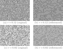
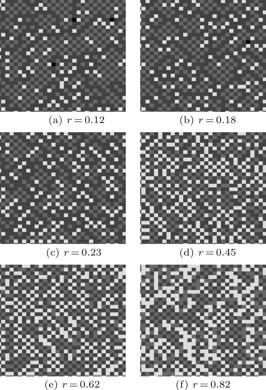
By incorporating the three diagrams of gca, gcb, and fa against r, one can quantitatively understand the properties of the global cooperation frequency fc as a function of r. Here, we only analyze qualitatively the evolution behaviors of A- and B-type agents. Making a comparison between Fig. 2 and the corresponding figure of fc given by Wang et al., [30] we find that (i) the global cooperation frequency fc at fa0 = 1.0 in our model is almost the same as theirs, and (ii) fc for other fa0 is also very similar to theirs, except for the range of 0 < r < 1/4, in which it has three splitted levels in our system, in contrast to only one in the system with pure A-type agents. It follows from Ref. [30] that the typical equilibrium structure of the strategy distribution in the ESG with pure A-type agents is something like a chessboard with some embedded “ C-lines” in the range of 0 < r < 1/4 or a chessboard-like background with small sparsely-embedded “ C-segments” in the range of 1/4 < r < 1/2, while it is also like a chessboard but with a few “ D-segments” in the range of 1/2 < r < 3/4 or with “ D-lines” in the range of 1/4 < r < 1. Here, the four intervals of r, (0, 1/4), (1/4, 1/2), (1/2, 3/4), and (3/4, 1.0), can be called the main ones. Obviously, in a chessboard-like background, the agent adopting D-strategy will have higher payoff than the one using the C-strategy. Thus, B-type agents will take the D-strategy position in the chessboard-like pattern of strategies; otherwise, they will have a high probability of suffering successive failures in the evolutionary game and have to change into A-type ones. Of course, in the small-r case, B-type agents also have a little probability of occupying the inner sites of “ C lines” embedded in the chessboard and survive finally. The above argument can be verified by the snapshots in the equilibrium state, as illustrated in Fig. 5, in which we make a comparison between the original scattergram of the strategy and type distribution and the referenced one without regard to the agent type. Figures 4(c) and 4(d) indicate that all of the B-type agents will adopt the D-strategy if r > 0.2 and only a few of them may use the C-strategy if 0 < r < 0.2. On the other hand, figure 2 shows that each of the first three main intervals will separate further into two or three secondary ones and, among the same main interval, the fraction of B-type agents for each secondary level increases with increasing r. Since one B-type agent occupying the D-strategy position of the chessboard pattern can compel four A-type agents in his neighborhood that they have to take over the C-strategy positions, the relative cooperation frequency gca for different secondary levels will be enhanced abnormally with the increase of B-type agents in the same main interval of r, as illustrated in Figs. 4(a) and 4(b). Especially, in the main interval of 0 < r < 1/4, the slight decline in the fraction of A-type agents can cause a significant increase in gca but a little decrease in gcb, which results in an abnormal improvement of the global cooperation frequency fc for different secondary levels along with increasing r (see Fig. 2).
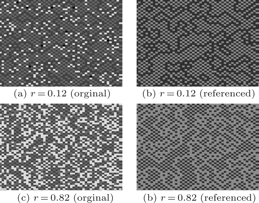 | Fig. 5. Snapshots of spatial patterns of cooperators and defectors for different cost-to-benefit ratios: (a) and (b) r = 0.12 and (c) and (d) r = 0.82. Besides, panels (a) and (c) are original scattergrams of the strategy and type distribution, which consist of A-type cooperators (blue), B-type cooperators (black), A-type defectors (red), and B-type defectors (yellow); while, panels (b) and (d) are referenced scattergrams of the strategy distribution without regard to the agent type, which consist of cooperators (dark green) and defectors (orange). Here, the other model parameters are the same, ν T = 3 and fa0 = 0.5. Obviously, almost all of B-type agents will occupy the D-strategy sites in the chessboard-like pattern of strategies; while in the small-r case, a few of the B-type agents might also occupy the inner sites of “ C lines” (dark green) embedded in the chessboard. |
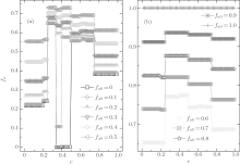
Next, we investigate the case with a moderate value of ν T. Here, we select ν T = 36 as an example. The global cooperation frequency fc as a function of r for different fa0 is demonstrated in Fig. 6. We again observe that fc is of a discontinuous plateau structure. As a contrast to the ν T = 3 case, the discontinuous jump in the global cooperation frequency fc at r = 1/6 disappears in this case, and the phenomenon that the values of the secondary levels abnormally enhance with increasing r in the interval of 0 < r < 1/4 does not occur any more. The disappearance of the secondary jump at rc = 1/6 indicates that the configuration C(1C3D) cannot form in the range of 0 < r < 1/6 when ν T = 36. It is not surprising because the configuration C(1C3D) is difficult to form in rich-C background and figure 6 shows fc > 0.64 at 0 < r < 1/6. While, new discontinuous transitions at rc = 1/3 and rc = 2/5 can occur in this case if fa0 ≤ 0.2 and one more new jump will arise at r = 2/3 if fa0 = 0. According to Table 2, the competition between the configurations C(0C4D) and D(2C2D) leads to the jump at rc = 1/3, while that between the configurations C(1C3D) and D(2C2D) causes the jump at rc = 2/5. These configurations, such as C(0C4D), C(1C3D), and D(2C2D), can easily form in rich-D background. Figure 6 shows that fc < 0.5 in the range of 1/4 < r < 1/2 only for fa0 ≤ 0.2. So, the analyses on the basis of the local stability of configurations are in accordance with these observations. Moreover, when 1/2 < r < 1, fc in this case is the same as that in the ν T = 3 case, and when 1/4 < r < 1/2, fc is also similar to that in the ν T = 3 case, except for small fa0 (i.e., fa0 ≤ 0.2 ); while for 0 < r < 1/4, the value of fc is distinctly larger than that in the ν T = 3 case.
 | Fig. 6. The equilibrium cooperation frequency fc as a function of the cost-to-benefit ratio r at ν T = 36. Each fc exhibits a discontinuous steplike structure for an arbitrary composition fa0. And the value of fc is independent of fa0 in the range of 1/2 < r < 1. |
In this case, the equilibrium fraction of A-type agents fa also shows a discontinuous plateau structure, as demonstrated in Fig. 7. Besides the three main jumps occurring at r = 1/4, 1/2, and 3/4, some new discontinuous transitions arise within the first three main intervals, but which will disappear once fa0 is beyond a certain value. In the first main interval of 0 < r < 1/4, there is a discontinuous jump occurring at r = 1/5 and this jump will disappear if fa0 ≥ 0.9; in the second main interval of 1/4 < r < 1/2, there are two discontinuous jumps arising respectively at r = 1/3 and r = 2/5, but which will disappear if fa0 ≥ 0.7; and similarly, in the main interval of 1/2 < r < 3/4, one can also observe two inapparent jumps emerging at r = 3/5 and r = 2/3 when fa0 ≤ 0.6. Moreover, at a given r, the value of fa always increases consistently with the increase of fa0, and except for fa0 = 0, 0.1, and 1.0, fa for other fa0 has the maximum value in the main interval of 1/4 < r < 1/2 and the minimum value in the main interval of 0 < r < 1/4. In more detail, when fa0 ≤ 0.5, the level of fa for the secondary range of 1/3 < r < 2/5 has the minimum value within the main interval of 1/4 < r < 1/2, while it has the maximum value for the secondary range of 3/5 < r < 2/3 within the main interval of 1/2 < r < 3/4. More intriguingly, when fa0 = 0 and 0.1, the value of fa − fa0 is equal to zero in the range of 1/3 < r < 2/5, in other words, all B-type agents cannot change into A-type ones. While the value of fa is very close to zero in the range of 2/5 < r < 1/2 if fa0 = 0, namely, only a tiny proportion of B-type agents can become A-type ones under such a situation. It is also worth noting that when fa0 = 1.0, fa is consistently equal to unity, independent of r. It is thus concluded that in the system initializing with pure A-type agents, all A-type agents cannot change into B-type ones. similar to the above ν T = 3 case, the equilibrium fraction of A-type agents fa is always larger than (or equal to) the corresponding initial quantity fa0 and the net difference between them consistently decreases with increasing fa0.
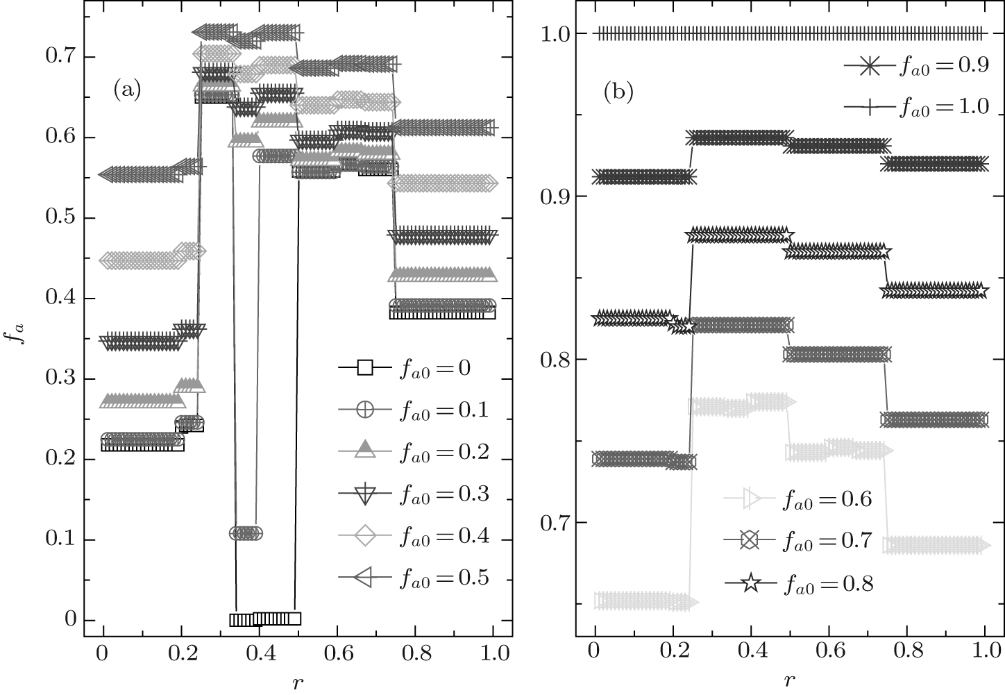 | Fig. 7. The equilibrium composition fa versus the cost-to-benefit ratio r at ν T = 36. Each fa exhibits a discontinuous steplike structure for each initial composition fa0, and the number of plateaux has relation with the value of fa0. Especially, fa ≃ fa0 for fa0 = 0 in the range of 1/3 < r < 1/2, and it is also the case for fa0 = 0.1 in the range of 1/3 < r < 2/5. |
Now we investigate the relative cooperation frequencies gca and gcb. In this case, both gca and gcb are also of plateau structures, as shown in Fig. 8. gca has eight plateaux when fa0 ≤ 0.5; however, with the increase of fa0, the secondary discontinuous transitions at r = 1/5, 1/3, 2/5, and 3/5 will gradually disappear, and the number of plateaux finally decreases to 4 when fa0 = 1.0. Moreover, in the range of r > 0.5 and 1/4 < r < 1/3, the equilibrium value of gca decreases with increasing fa0; while in the remaining range, gca first increases and then decreases with the increase of fa0, and the maximum value of gca is attained at fa0 ≃ 0.6 in the range of 0 < r < 1/4, at fa0 ≃ 0.3 in the range of 1/3 < r< 2/5, and at fa0 ≃ 0.2 in the range of 2/5 < r < 1/2, respectively. It is also worth noting that when fa0 ≤ 0.2, the value of gca for large r is larger than 0.8, namely, most A-type agents will adopt the C-strategy in such situations. Meanwhile, we observe that gcb = 0 for all fa0 ≥ 0.1 in the range of r > 2/5, namely, all B-type agents will adopt the D-strategy to survive under the large-r situation. In the main range of 0 < r < 1/4, the value of gcb decreases from about 0.8 to 0 with the increase of fa0; while two secondary discontinuous jumps occur at r = 1/6 and r = 1/5, which will become more and more obvious with increasing fa0, and the levels of gcb for different secondary plateaux decrease along with r. Especially, when fa0 = 0, we observe gcb ≃ 0.5 in the range of 1/3 < r < 1/2, and when fa0 = 0.1, gcb ≃ 0.45 in the range of 1/3 < r < 2/5.
 | Fig. 8. The relative cooperation frequencies gca and gcb versus the cost-to-benefit ratio r at ν T = 36. It is shown that both gca and gcb have a discontinuous steplike structure for each initial composition fa0. gcb decreases with fa0 in the range of 0 < r < 1/2, while it consistently equals zero in the range of 1/2 < r < 1. gca always has a non-zero value for arbitrary r. Moreover, with increasing fa0fc first increases and then decreases in the range of 0 < r < 1/2, and it consistently decreases with the increase of fa0 in the range of 1/2 < r < 1. |
Finally, by combining the relative cooperation frequencies gca and gcb with the equilibrium composition fa, we briefly interpret the above-mentioned behaviors of the global cooperation frequency fc that differ from those in the ν T = 3 case. In the ν T = 36 case, with the increase of r, there are slight increases both in fa and gca around the discontinuous point r = 1/5, but a considerable decrease of gcb also happens at the same time. It is the case for all fa0 ≤ 0.9. Thus, before and after the transition point r = 1/5, the global cooperation frequency fc for different secondary levels decreases slightly along with r. Moreover, for fa0 = 0, almost all B-type agents cannot change into A-type ones in the range of 1/3 < r < 1/2 and, thus in such a situation our system is equivalent to the pure B-type agent system with the unconditional imitation rule, in which fc ≃ 0.5 and an inapparent jump occurs at r = 2/5.[41] While for fa0 = 0.1, all B-type agents cannot change into A-type ones in the range of 1/3 < r < 2/5 and then our system is identical to the heterogenous system with a fixed composition of A- and B-type agents, [46] in which fc ≃ 0.45.
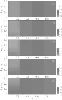
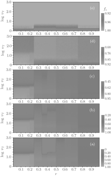
In this section, we discuss the overall dependence of the evolution behaviors of the heterogenous systems on the upper limit of tolerance ν T (ν T ≥ 2). We select several values of fa0 as examples to show the equilibrium cooperation frequencies and the equilibrium fraction as functions of r and ν T. Figure 9 shows the equilibrium cooperation frequency fc as a function of r and ν T for different values of fa0. Obviously, as indicated by the contour lines in parallel with the ν T-axis, each fc shows a plateau structure with three main discontinuous transitions at r = 1/4, 1/2, and 3/4, respectively. Besides, there are also several secondary discontinuous transitions occurring in fc in the first two main intervals of 0 < r < 1/4 and 1/4 < r < 1/2, but which will gradually disappear with the increase of ν T as well as fa0, and one can easily find the number of plateaux in fc against r for an arbitrary value of ν T by making a horizontal cut at this ν T-value. On the other hand, figure 9 also indicates that the value of fc increases consistently with increasing ν T in the interval of 0< r< 1/4, while it is independent of ν T in the interval of 3/5< r< 1.
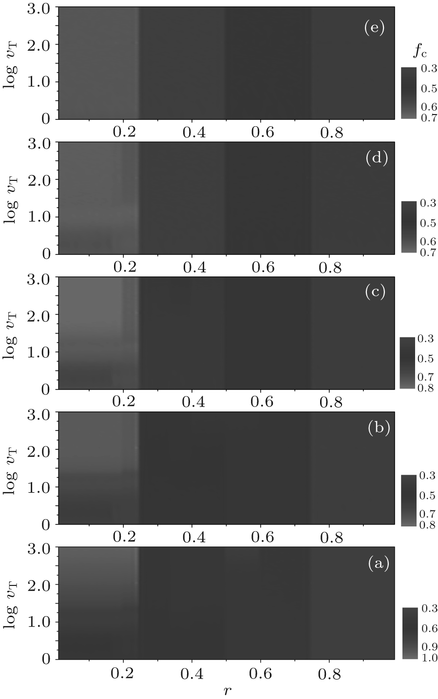 | Fig. 9. The equilibrium cooperation frequencies fc versus the cost-to-benefit ratio r versus the upper limit of tolerance ν T for different fa0 are plotted as a contour map. Here, (a) fa0 = 0; (b) fa0 = 0.3; (c) fa0 = 0.5; (d) fa0 = 0.8; and (e) fa0 = 1.0. fc shows discontinuous steplike structures and neighboring plateaux are divided by several distinct contour boundaries at some particular values of r, i.e., the transition points. |
Figure 10 illustrates the equilibrium composition fa as a function of r and ν T for different values of fa0, which is also of an obvious plateau structure. For small fa0, i) fa first keeps a constant independent of ν T until ν T is beyond a certain value, and it then rapidly decays to the initial value fa0 with increasing ν T in the ranges of 0 < r < 1/4 and 1/3 < r < 1/2; (ii) fa slightly decreases to a steady value much larger than fa0 with increasing ν T in the range of 3/5 < r < 1; and iii) fa consistently decreases to a non-zero value finally in the remaining range of r. For very large fa0, fa first increases with increasing ν T and then rapidly reaches to a steady value. For mediate fa0, fa first keeps a constant independent of ν T and then rapidly decays to the steady value fa0 eventually in the range of 0 < r < 1/4, while it first increases with the increase of ν T and then slightly decays to a non-zero value finally in the range of 1/4 < r < 1. On the other hand, the quantity of fa increases with the increase of fa0. Moreover, when ν T is small (say, ν T< 10), fa is close to unity in the range of 0 < r < 1/4, namely, most of the agents are A-type ones and adopt the memory-based updating rule; while in the remaining range of r, one can observe that fa ≥ 0.7 in the range of 1/4 < r < 1/2, fa ≥ 0.6 in the range of 1/2 < r < 3/4, and fa ≥ 0.5 in the range of 3/4 < r < 1, and thus, at least half of the agents will take the A-type role even under the fa0 = 0.0 and r > 3/4 condition. When ν T is large (say, ν T > 100 ), we find that in the range of 0 < r < 1/4, fa ≃ fa0, namely, it is almost impossible for an agent changing its type, and it is also the case for the fa0 ≤ 0.3 system in the range of 1/3 < r < 1/2; while in the remaining range of r, fa > fa0, that is, a certain percentage of B-type agents change into A-type ones finally. It should also be pointed out that a small percentage of A-type agents can change into B-type ones only when ν T is small (see, e.g., panel (e) in Fig. 10).
 | Fig. 10. The equilibrium composition fa versus the cost-to-benefit ratio r versus the upper limit of tolerance ν T for different fa0 are plotted as a contour map. Here, (a) fa0 = 0; (b) fa0 = 0.3; (c) fa0 = 0.5; (d) fa0 = 0.8; and (e) fa0 = 1.0. fa shows discontinuous steplike structures and neighboring plateaux are divided by several distinct contour boundaries at some particular values of r, i.e., the transition points. |
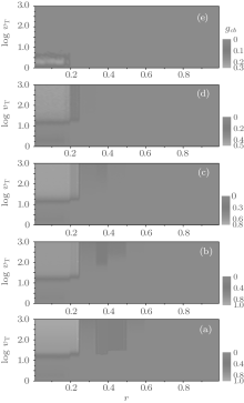
Finally, we also analyze the relatively cooperation frequencies gca and gcb. As illustrated in Fig. 11, for arbitrary ν T and fa0, gca as a function of r is of an obvious plateau structure with three main discontinuity points at r = 1/4, 1/2, and 3/4, respectively. In each of the first three main intervals of r (namely, 0 < r < 1/4, 1/4 < r < 1/2, and 1/2 < r < 3/4), the cooperation level will split further into several secondary plateaux. For large fa0, say fa0 = 1.0, gca first decreases with the increase of ν T and soon decays to a steady value, which is independent of the value of r. While for small or moderate values of fa0, the evolution of gca depends on the value of ν T as well as the value interval of r. Some remarkable features are listed as follows: a) the value of gca will reach to a steady value at large ν T; b) with ν T increasing from 2 to 1000, gca rapidly increases from the beginning in the range of 0 < r < 1/4 and 3/4 < r < 1, while it first decreases slightly and then rapidly increases to a steady value; c) gca has a maximum value at about ν T = 15 when 0 < r < 1/4; and d) when 1/3 < r < 1/2 and fa0 = 0, gca = 0 at large ν T. As a contrast to A-type agents, the cooperative behavior of B-type ones is quite simple, as illustrated in Fig. 12. For large r and fa0, gcb is almost equal to zero (namely, all B-type agents will adopt the D-strategy finally); while, only for small r and large ν T, gcb has a non-zero value.
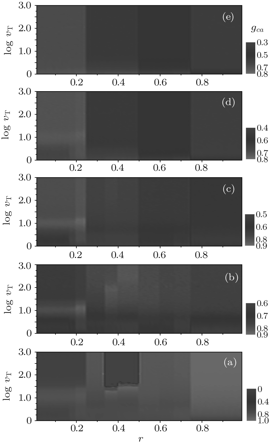 | Fig. 11. The relative cooperation frequency gca versus the cost-to-benefit ratio r versus the upper limit of tolerance ν T for different fa0 is plotted as a contour map. Here, (a) fa0 = 0; (b) fa0 = 0.3; (c) fa0 = 0.5; (d) fa0 = 0.8; and (e) fa0 = 1.0. gca shows discontinuous steplike structures and neighboring plateaux are divided by several distinct contour boundaries at some particular values of r, i.e., the transition points. |
 | Fig. 12. The relative cooperation frequency gcb versus the cost-to-benefit ratio r versus the upper limit of tolerance ν T for different fa0 is plotted as a contour map. Here, (a) fa0 = 0; (b) fa0 = 0.3; (c) fa0 = 0.5; (d) fa0 = 0.8; and (e) fa0 = 1.0. It is shown that gcb equals zero for almost all experimental parameters, except for large ν T and small r. |
In this work, we proposed an ESG in heterogenous agent systems with co-evolutionary strategies and updating rules. In the game systems, there are two types of agents: A-type and B-type. A-type agents adopt the memory-based rule to update their strategy while B-type ones use the unconditional imitation rule. Moreover, either type of agents can change into the other type if they suffer sequential failures beyond their upper limit of tolerance. We focused on the influences of the upper limit of tolerance and the initial composition of agents on the cooperative behavior of such heterogenous agent systems. Considering a simple ESG with the same upper limit of tolerance for all agents, we then studied its cooperative behavior by performing numerical simulations on a 2D square lattice with periodic boundary conditions.
It is found that the cooperation frequency fc against r exhibits a steplike discontinuous plateau structure, and that the number of plateaux is independent of the upper limit of tolerance ν T as well as the initial composition fa0. Generally, three main discontinuous transitions exist occurring at r = 1/4, 1/2, and 3/4, respectively, which divide the plateaux into four groups. In the first two groups, the plateaus may further split into several secondary discontinuous ones under some parameter conditions, and these secondary discontinuous jumps will gradually disappear with the increase of ν T as well as fa0. More intriguingly, in the first main interval of 0 < r < 1/4, the levels of secondary discontinuous plateaux abnormally increase with increasing r when ν T is small, say ν T = 3. Moreover, the value of fc increases consistently to a steady quantity with increasing ν T in the interval of 0 < r < 1/4 and it is just to the contrary in the interval of 1/4 < r < 3/4, while it is independent of ν T in the interval of 3/5 < r < 1.
We also observed that the equilibrium composition fa as a function of r is of an obvious plateau structure. Besides, the quantity of fa depends crucially on the initial composition fa0, the upper limit of tolerance ν T, and the cost-to-benefit r. Firstly, fa increases with the increase of fa0. Secondly, when ν T is small, either type of agent can change their role into the other one, but the possibility of B-type agents changing into A-type ones is larger than that of the inverse process and, thus, for small or moderate fa0, fa is always larger than fa0; when ν T is very large, an agent changing its type becomes impossible in the range of 0 < r < 1/4 and it is similar for the fa0 ≤ 0.3 system in the range of 1/3 < r < 1/2, while in the remaining range of r, a certain percentage of B-type agents will eventually change into A-type ones. More interestingly, when ν T is small, almost all agents will be A-type ones in the range of 0 < r < 1/4 and more than half of agents will take the A-type role even in the large-r case, independent of the initial composition fa0.
In order to understand thoroughly our ESG system, we further analyzed the relative cooperative behavior of either type of agent. The relatively cooperation frequency gca as a function of r is of an obvious plateau structure with three main discontinuous jumps at r = 1/4, 1/2, and 3/4, respectively, and the cooperation level among the main interval of r will split further into several secondary plateaux. The quantity of gca depends on the value of ν T as well as the value of r. With increasing ν T, gca first increases rapidly and reaches to a steady value at large ν T. It is also worth noting that gca has a maximum value at about ν T = 15 when 0 < r < 1/4. Besides, we observed gca = 0 at large ν T when 1/3 < r < 1/2 and fa0 = 0. The relatively cooperative frequency gcb of B-type agents has relatively simple behavior. When ν T is small, all B-type agents adopt the D-strategy in the range of 1/5 < r < 1, i.e., gcb = 0, while only very few B-type agents take the C-strategy in the remaining range of 0 < r < 1/5. When ν T is large, we also observed gcb = 0 in the range of 3/5 < r < 1 but gcb has a non-zero value in the range of 0 < r < 3/5. Thus, for the practical case with small ν T, B-type agents almost contribute nothing to the cooperation level of the system.
Furthermore, numerical simulations on hexagonal and cubic lattices also exhibit the above-mentioned similar phenomena. So, the key feature that fc versus r is of a plateau structure is typical of ESG with the mixed unconditional imitation and memory-based updating rules on regular lattices. This work is helpful for understanding in depth the ESG of heterogenous agent systems.
| 1 |
|
| 2 |
|
| 3 |
|
| 4 |
|
| 5 |
|
| 6 |
|
| 7 |
|
| 8 |
|
| 9 |
|
| 10 |
|
| 11 |
|
| 12 |
|
| 13 |
|
| 14 |
|
| 15 |
|
| 16 |
|
| 17 |
|
| 18 |
|
| 19 |
|
| 20 |
|
| 21 |
|
| 22 |
|
| 23 |
|
| 24 |
|
| 25 |
|
| 26 |
|
| 27 |
|
| 28 |
|
| 29 |
|
| 30 |
|
| 31 |
|
| 32 |
|
| 33 |
|
| 34 |
|
| 35 |
|
| 36 |
|
| 37 |
|
| 38 |
|
| 39 |
|
| 40 |
|
| 41 |
|
| 42 |
|
| 43 |
|
| 44 |
|
| 45 |
|
| 46 |
|
| 47 |
|