In recent years, the dynamics of magnetization driven by a spin-polarized current has received considerable attention in ferromagnetic nanowires.^{[1– 5]} In the presence of a spin-polarized current, the Landau– Lifshitz– Gilbert equation^[6] should be modified to describe the magnetization dynamics in a ferromagnet. Three kinds of excited magnetic states have been found in the ferromagnetic nanowire, namely: the spin wave, the dynamic soliton, and the magnetic domain wall.^[7] In the ferromagnetic nanowire, the interaction of spin waves is attractive and its instability results in the dynamic soliton or domain wall, which is characterized by the localization in some sufficiently small region and moves while retaining its shape.

The domain wall, i.e., the topological magnetic soliton, and its properties have been studied in the pioneering work of Bloch, Landau, Lifshitz, and Tonks.^[8] Because the domain wall describes two degenerated states of magnetization, the research of the domain wall can be applied technologically to race track memory and logic devices.^{[9, 10]} Therefore, the magnetic field or spin polarized current driven dynamic properties of the domain wall have been extensively studied in ferromagnetic nanowires.^{[4, 5, 11– 19]} With the detection of magnon excitation, ^{[20, 21]} the motion of magnetization of a dynamic soliton has been investigated in confined ferromagnetic materials.^{[20– 25]}

Nowadays, the external field^[26] and the spin-polarized current^[27] are the main driven forces for the dynamics of magnetization. The magnetization orientation of a nanoscale ferromagnet can be manipulated by a spin-transfer torque and some unique phenomena have been observed for the magnetization motion. With the spin-transfer torque effect, the optimal time-dependent current pattern for the domain wall dynamics^[28] was investigated in a ferromagnetic nanowire. Recently, more attention has been directed to the magnetization motion caused by a spin-transfer torque in the polarizing reference layer. In this case, the spin-transfer torque could destabilize the reference layer and cause its precession.^{[29– 34]} Generally, the thickness of the fixed reference layer is required to be much thicker than that of the free layer. However, recent experiments have demonstrated that the spin torque could rotate the magnetization of the reference layer and trigger radio frequency oscillations.^{[32– 34]}

In this paper, with a destabilized reference layer, we investigate the nonlinear dynamics of magnetic soliton and the magnon density properties in an uniaxial anisotropic ferromagnet driven by a spin-transfer torque. Our results show that the spin polarized current affects the magnon density distribution, which is described by the amplitude of soliton. We also find that each magnetic soliton exhibits no changes in both velocity and magnon density distribution in the process of two solitons collision.

Owing to the Joule heating effect, magnetization is rotated at a high enough current density, and this in turn results in the interaction of the magnetization in the free and reference layers via the spin-transfer torque effect. Therefore, we can assume that the reference layer is partially fixed in the model system. With this consideration, the magnetization dynamics of the free layer takes the form of Landau– Lifshitz– Gilbert equation with a spin-transfer torque

where γ is the gyromagnetic ratio, α is the Gilbert damping parameter, and the effective magnetic field H_eff is the vector sum of the exchange field, the anisotropy field, and the applied external field. For the perpendicular anisotropy case, the effective magnetic field takes the form , where A is the exchange constant, H_K denotes the anisotropy coefficient, H is the applied external field, and e_z is the unit vector along the z axis. The last term T_S of Eq.  (1) denotes the spin-transfer torque, and we generally takes the Slonczewski torque, i.e., T_S= γ M_sA_j[m× (m× m_R)], with A_j= Pj_eℏ /(2| e| d), m ≡ M/M_s, M_s being the saturation magnetization, and m_R being the dimensionless magnetization of the reference layer. Here, P is the spin polarization, j_e is the current density, e is the magnitude of electron charge, and d is the thickness of the free magnetic layer.

When the hard axis of the reference layer is along the z axis, the magnetization can rotate in the x– y plane, which can be assumed to have the form m_R= m× (m_xe_x + m_ye_y). This implies that the spin waves can be excited in the free layer. With the assumption ψ ≡ m_x+ im_y and without damping, under the long-wavelength approximation, ^[7] equation  (1) reduces to

where time t and space coordinate x have been rescaled by the characteristic time t₀= 1/(γ M_s) and length , respectively. The other parameters are g= (h_K − a_j)/2 and ω = h_K+ h₁-a_j, with h_K= H_K/M_s, h₁= H/M_s, and a_j= A_j/M_s. From Eq.  (2), we observe that the parameter g is similar to the s-wave scattering length in Bose– Einstein condensates, ^[35] which denotes the interatomic interaction. In Bose– Einstein condensates, the interatomic interaction can be tuned experimentally by utilizing the Feshbach resonance, ^[36] even including its sign. In ferromagnetic nanowires, the spin-polarized current plays the same role and admits different states for magnetization, as shown later.

Equation (2) admits two obvious solutions, i.e., ψ = 0 and ψ = A_ce^{i(ω _ct-k_cx)}, here ω _c and k_c are the frequency and the wave number, respectively. The former corresponds to the ground state m= (0, 0, 1), and the latter denotes the spin wave solution of magnetization. The attractive interaction of spin waves results in instabilities, which can explain the appearance of a spatially localized topological or dynamic soliton. As shown below, analytical bright and dark soliton solutions of magnon density can be constructed for g> 0 and g< 0, respectively. These solutions can display some results by adjusting the spin current.

The Hirota method^[37] is an effective and straightforward technique to solve nonlinear equations. With this technique, the one- and two-bright soliton solutions of magnon density are easily obtained for g> 0, which denotes the critical current condition a_j< h_K. These solutions can be well expressed by the magnon function ψ , which takes the form of bright soliton of Eq.  (2). The one-soliton solution of Eq.  (2) takes the form

where , and . Here the parameter ξ is an arbitrary complex parameter, and subscripts R and I represent the real and the imaginary parts, respectively. The solution in Eq.  (3) denotes a dynamic precession of magnetization on the ground state background. The magnetic soliton moves with velocity v= -2ξ _I, and the components m_x and m_y precess around m_z with the transverse amplitude 1/(2β cosh θ ) affected by the spin current a_j and the frequency controlled by the spin current and the external field. Along the soliton propagation direction, i.e., θ = 0, the magnon density reads . This demonstrates that the magnon density distribution can be adjusted by the spin current, as shown in Figs.  1(a) and 1(b). The magnon density peak increases with increasing current. When the small perturbations are included into the magnetization motion, the dynamic solitons can evolute into the uniform magnetization by continuous deformation. These results imply that the excited ferromagnet makes a transition to the ground state.

With the same procedure, we obtain the analytical two-soliton solution of Eq.  (2)

where

here , with p_j = α _j+ i β _j, j= 1, 2 and . The solution in Eq.  (4) represents a general scattering process of two magnetic solitons with different central velocities v₁ and v₂. The collision dynamics of two magnetic solitons is plotted in Fig.  1(c). The properties of the two dynamic solitons interaction can be clarified by the asymptotic behavior of the soliton solution in Eq.  (4). For this purpose, we study the asymptotic forms of Eq.  (4) in limits t→ -∞ and t→ ∞ .

Before collision (t→ -∞ ), we havea) soliton 1 (θ ₁≈ 0, θ ₂→ -∞ )

b) soliton 2 (θ ₂≈ 0, θ ₁→ ∞ )

After collision (t→ ∞ ), we havea) soliton 1 (θ ₁≈ 0, θ ₂→ ∞ )

b) soliton 2 (θ ₂≈ 0, θ ₁→ -∞ )

The above formulas clearly demonstrate that only center and phase shifts occur in the process of the two solitons collision. This result indicates that the collision of two solitons is elastic, as illustrated in Fig.  1(c).

Fig.  1.

	Figure Option ViewDownloadNew Window
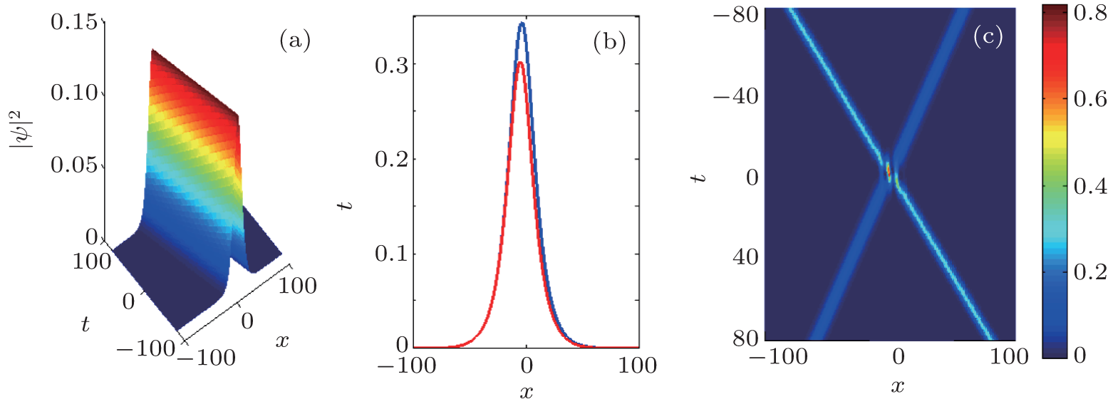	Fig.  1. (a) and (b) Evolution of bright soliton of magnon density with different currents (blue: 0.035 and red: 0.01 ). The other parameters are ξ R= 0.1, ξ I= 0.12, and hK= 0.12. (c) Soliton collision with parameters k1= 0.45, hK= 0.42, aj= -0.75, h1= -0.9, p1= 0.2+ i 0.365, and p2= 0.3-i 0.5.

When the current exceeds the critical value, i.e., g< 0, the nonlinear dynamics of magnetization are different from the above discussion. The magnon density admits the dark soliton solution, which can also be well expressed by the magnon function ψ . Employing the Hirota method, we obtain one-soliton solution

where η ₀= p₀x-Ω ₀t+ ξ ₀, η ₁= p₁x+ Ω ₁t+ ξ ₁, and . Here the parameters ξ ₀ and ξ ₁ are real constants. The other parameters are , and . From the solution in Eq.  (9), we easily find two special cases, i.e., C= ± 1. When C= 1, the solution (9) reduces to spin wave solution characterized by phase velocity Ω ₀/p₀ and frequency Ω ₀. The transverse amplitude and frequency of the spin wave are also affected by the spin current. The distribution of magnon density is uniform, while controlled by the spin current. When C= -1, the solution in Eq.  (9) becomes tanh (η ₁/2), where η ₁= p₁(x+ 2p₀t). This result describes a nonuniform distribution of magnon density in the space. The velocity and the width of the soliton are constant, i.e., -2p₀ and 1/p₁, respectively. The soliton depth, i.e., 8λ /| h_K-a_j | , also depends on the current. As shown in Fig.  2(a), it describes a dark soliton solution for magnon density | ψ | ². While in the case of g→ ∞ , the direction of magnetization is along the z axis, i.e., ψ → 0 and m→ (0, 0, 1), which displays the ground state of magnetization.

In the same way, we can obtain the two-soliton solution

where

here j= 1, 2, and all the parameters have been obtained in the previous section

Fig.  2.

	Figure Option ViewDownloadNew Window
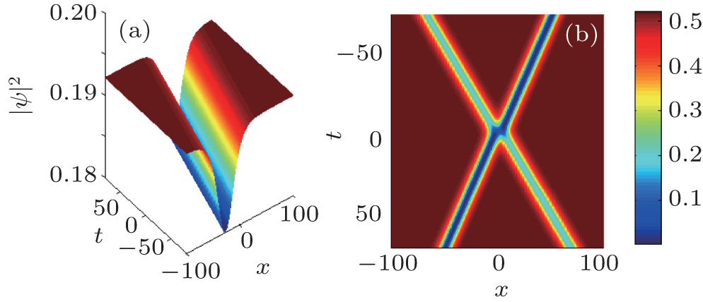	Fig.  2. (a) Evolution of dark soliton of magnon density with parameters hK= 0.12, aj= 0.85, h1= 0.12, ξ 0= 0.1, ξ 1= 0.05, p0= 0.02, p1= 0.1, and λ = 0.08. (b) Two solitons collision with parameters hK= 0.62, aj= 1.85, ξ 0= 0.5, ξ 1= 0.6, λ = 0.08, h1= 0.8, p0= 0.3, p1= 0.32, and p2= 0.4.

To well understand the dynamics in Eq.  (10), we plot the grey soliton solution to describe the two dark solitons of magnon density, which shows the general scattering process of the two solitons. In Fig.  2(b), we see that each magnon density exhibits no changes in either velocity and width after the collision. There is only a shift for each soliton center. In fact, the solution  (10) represents two magnon density solitons collision under the spin wave background. The asymptotic forms of Eq.  (10) in limits t→ -∞ and t→ ∞ are similar to those of the solution of Eq.  (9).

Before collision (limit t→ -∞ ), we havea) soliton 1 (η ₁≈ 0, η ₂→ -∞ )

b) soliton 2 (η ₂≈ 0, η ₁→ ∞ )

After collision (limit t→ ∞ ), we havea) soliton 1 (η ₁≈ 0, η ₂→ ∞ )

b) soliton 2 (η ₂≈ 0, η ₁→ -∞ )

where , and δ ₀= ln B₁₂. The above asymptotic behavior analysis confirms that there is no change for the magnon distribution of each dark soliton in the process of soliton collision. However, from Eqs.  (11)– (14), we find a phase exchange δ ₀/2 for the collision, which shows the elastic collision of the two solitons.

In summary, we have investigated current-induced magnetic soliton solutions in a perpendicular ferromagnetic anisotropy nanowire. Our results show that the magnon density distribution admits bright and dark soliton states by adjusting the current. The magnon density can be modulated by the spin-polarized current, which is described by the soliton amplitude. Furthermore, we find that the two-soliton solution is in fact a combination of two single solitons and each magnon density soliton exhibits no changes in either velocity and width before and after the collision. This clearly shows that the soliton collision is elastic.