The study is conducted to predict the fluid transients in a system comprised of a horizontally-mounted pipe of constant cross-sectional area, in which a fluid is initially flowing at a constant velocity. One tested pipe is taken to be connected to an upstream tank and a downstream tank, and a shut-off valve is mounted in the middle of the pipeline, as shown in Fig. 1.

Fig. 1.

	Figure Option ViewDownloadNew Window
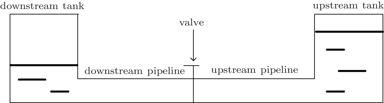	Fig. 1. Tank– pipeline– valve system.

A mathematical model for pressure and flow transients following a rapid closure of the valve (as illustrated in Fig. 1) is presented, in which models of the friction item are incorporated. Based on the principle of fluid dynamics, the basic equations applied to simulate the transient pipeline flow can be obtained from the continuity equation and the motion equation.^{[14, 15]} The continuity equation is

The motion equation is

Here, c₀ is the acoustic velocity of the liquid medium; p and q are the transient pressure and flow rate at some point along the pipeline, respectively; t is the time variable; x is the space variable; ρ is the density of the fluid; r is the inner radius of the pipeline; F(q) is the friction item; g is the gravitational acceleration; and θ ₀ is the angle between the pipeline and the horizon.

In Eq. (2), the friction item F(q) can be described as the sum of steady state friction item F₀ and frequency-dependent unsteady friction item F_f,

By using the Fourier transform, the friction item F(q) can be written as

where μ is the dynamic viscosity of the fluid; J₀ and J₁ are the zero-order and the first-order Bessel functions, respectively; and λ is given by

with ν being the kinematic viscosity of the fluid, ω the angular frequency, and γ a dimensionless frequency, which is given as

In the case of laminar flow, the steady friction item F₀ in Eq. (3) can be calculated as

The frequency-dependent friction item F_f can be described as

where H(s) is the analytical model of the frequency-dependent friction item

The analytical model of the frequency-dependent friction item contains Bessel functions, which leads to complex calculations and inconvenience in operation.^[12] In order to simulate the pressure transients accompanying the friction in pipelines, a model is presented here which attempts to capture the key features but without being unduly complex. The approximate model H_app(s) can be described as the sum of a list of weighting terms,

where n_i and m_i are coefficients of the weighting function; and k is the number of weighting terms.

Trikha proposed three exponent weighting items to approximate the frequency-dependent friction items.^[16] The coefficients of the three weighting terms are listed in Table 1. The amplitude-frequency and phase-frequency characteristics of each weighting term are illustrated in Fig. 2. The x coordinate is dimensionless frequency γ . It can be seen from Fig. 2 that each weighting function of the frequency-dependent friction item is similar to a first-order high-pass filter.

Fig. 2.

	Figure Option ViewDownloadNew Window
	Fig. 2. Frequency characteristics of each weighting term for Trikha: (a) amplitude, (b) phase.

Table 1.

Table 1.

Table 1. Coefficients of three weighting terms for Trikha. i ni mi 1 26.4 1.0 2 200.0 8.1 3 8000.0 40.0

Table 1. Coefficients of three weighting terms for Trikha.

Comparisons of the frequency characteristics between approximate model H_app(s) (the dashed line) and analytical model H(s) (the solid line) are shown in Fig. 3. Here the y coordinate is the absolute value | H_app(s)| and | H(s)| . It can be obtained from Fig. 3 that the analytical model of the dynamic friction item, H(s), varies with the slope + 10 dB/dec, and in the higher frequency section, the phase angle is approximately 45° . The approximate model agrees with the analytical model H(s) in the low-frequency section when the dimensionless frequency γ is below 50; while the difference between H_app(s) and H(s) is obvious as the dimensionless frequency γ increases.

Fig. 3.

	Figure Option ViewDownloadNew Window
	Fig. 3. Comparisons of frequency characteristics between H(s) and Happ(s) from Trikha’ s model: (a) amplitude, (b) phase.

The biggest advantage of this method lies in that only the calculation result of the previous moment is stored without all integral results, which can greatly reduce the computer memory required and the calculation time. However, the iterative algorithm with an explicit increment of the flow rate at the moment still requires a large amount of computation time.

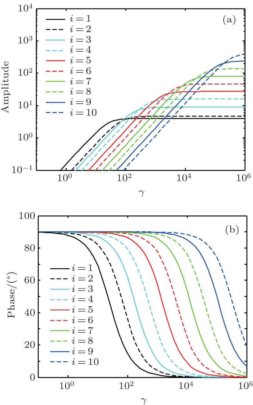
Kagama tried to reduce the error caused by using Trikha’ s model and used an approximate model with ten weighting terms instead.^[17] The coefficients of the ten weighting terms are listed in Table 2. Figure 4 shows the frequency characteristics of individual weighting terms. Comparisons of frequency characteristics between approximate model H_app(s) (the dashed line) and analytical model H(s) (the solid line) are shown in Fig. 5. It can be seen from Fig. 5 that the approximate model agrees with the analytical model H(s) in the low-frequency section when the dimensionless frequency γ is below 2000; while the difference between H_app(s) and H(s) is still obvious in the high-frequency section.

Fig. 4.

	Figure Option ViewDownloadNew Window
	Fig. 4. Frequency characteristics of each weighting term for Kagama: (a) amplitude, (b) phase.

Fig. 5.

	Figure Option ViewDownloadNew Window
	Fig. 5. Comparisons of frequency characteristics between H(s) and Happ(s) from Kagama’ s model: (a) amplitude, (b) phase.

Table 2.

Table 2.

Table 2. Coefficients of ten weighting terms for Kagama. i ni mi 1 26.3744 1.0 2 72.8033 1.16725 3 187.424 2.20064 4 536.626 3.92861 5 1570.60 6.78788 6 4618.13 11.6761 7 13601.1 20.0612 8 40082.5 34.4541 9 118153 59.1642 10 348316 101.590

Table 2. Coefficients of ten weighting terms for Kagama.

The approximate model proposed by Kagama has some improvements over Trikha’ s model. It has the characteristics of rapid solving speed and high accuracy. However, owing to a large number of items and a relatively close interval between the weighting functions in Kagama’ s approximate model, it is inconvenient for applications.^[12]

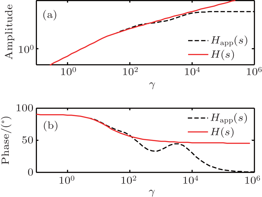
Taylor optimized the coefficients of Trikha’ s model and proposed an approximate model with four exponent weighting terms.^[18] The coefficients are listed in Table 3. Frequency characteristics of individual weighting terms for Taylor are illustrated in Fig. 6. Comparisons of frequency characteristics between approximate model H_app(s) (the dashed line) and analytical model H(s) (the solid line) are shown in Fig. 7. It can be seen from Fig. 7 that the approximate model agrees with the analytical model H(s) in the low-frequency section when the dimensionless frequency γ is below 5000; while the difference between H_app(s) and H(s) is obvious in the higher frequency section.

Fig. 6.

	Figure Option ViewDownloadNew Window
	Fig. 6. Frequency characteristics of each weighting term for Taylor: (a) amplitude, (b) phase.

Fig. 7.

	Figure Option ViewDownloadNew Window
	Fig. 7. Comparisons of frequency characteristics between H(s) and Happ(s) from Taylor’ s model: (a) amplitude, (b) phase.

Table 3.

Table 3.

Table 3. Coefficients of four weighting terms for Taylor. i ni mi 1 39.479 2.0141 2 298.2962 5.3946 3 2227.95 16.2591 4 88782.1 320.4853

Table 3. Coefficients of four weighting terms for Taylor.

From those preliminary studies, it can be observed that coefficients of each weighting function have the relationship of geometric series,

In order to predict more accurately the effect of the friction item on pressure transients inside pipelines, a new method using genetic algorithms (GAs) for parameter identification is described. Moreover, Li^{[19, 20]} has used GAs in parameter identification for a gas bubble model of low pressure oil-hydraulic pipelines.

Here four parameters of the approximate model of the frequency-dependent friction item need to be identified, including α , β , m₁, and n₁. For the optimization procedure, it is assumed that α , β , n₁ ∈ [1, 100], m₁ ∈ [0.1, 10] according to the weighting function coefficients obtained from the above three models. Each parameter is binary encoded, and the selection method of the best fit parameter is based on roulette.

The fitness function f of genetic algorithms is described as the sum of the least-square errors of amplitude-frequency and phase-frequency characteristics between approximate model H_app(s) and analytical model H(s),

where

In the genetic algorithms, the number of generations is 1000 and the population size of each generation is 100 in this paper. The crossover probability is 0.4 and the mutation probability is 0.005. Here the number of weighting terms k is set to be 7. The sensitivity of the predictions to the number of weighting terms selected will be considered later.

The aim is to perform a global search to obtain optimal parameters suitable for friction modeling. The identified results of four parameters are listed in Table 4.

Table 4.

Table 4.

Table 4. Identified parameters of the model. Identified parameter α β m1 n1 Value 3.5812 11.9733 2.2429 37.8463

Table 4. Identified parameters of the model.

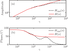
The comparison between analytical model H(s) (the solid line) and approximate model H_app(s) after identifying (the dashed line) is shown in Fig. 8. As can be seen, there is a good agreement between the two models in amplitude-frequency and phase-frequency characteristics, especially in the high frequency section.

Fig. 8.

	Figure Option ViewDownloadNew Window
	Fig. 8. Frequency characteristics of H(s) and Happ(s) with identified parameters (k = 7): (a) amplitude, (b) phase.

The parameters of the tested downstream pipeline obtained from Ref. [21] are listed in Table 5 and oil is the working fluid.

Table 5.

Table 5.

Table 5. Parameters of the tested downstream pipeline. Parameter Symbol Value Inner radius of pipeline r 4× 10− 3 m Length of pipeline L 20 m Density of hydraulic oil ρ 871 kg/m3 Acoustic velocity inside the fluid c0 1392 m/s Kinematic viscosity v 50.518 × 10− 6 m2/s

Table 5. Parameters of the tested downstream pipeline.

The number of weighting terms is determined by Eq. (19). The downstream of the pipeline is divided into N elements of equal length (N is 200), the simulation time step can be calculated from

By utilizing Eq. (16), the time constants of the first-order high-pass filter can be presented as

In the same way, the number of weighting terms can be acquired via Eq. (19) as

Hence, for the parameters of the downstream section of the pipeline, the number of weighting terms k is equal to 2.

Based on the mathematical model of transient pressure pulsations (shown in Eqs. (1) and (2)), the relevant simulation study on transient pressure pulsations in the downstream section of the pipeline is carried out using the finite difference method and the Matlab/Simulink platform. The flow rate and pressure in N elements along the pipeline are presented as vectors. According to the boundary condition, the flow rate in the element close to the valve is set to zero and the pressure in the element close to the tank is constant. See more technical details in Ref. [22].

The simulation parameters are also given in Table 5. The initial pressure close to the valve is 3 MPa and the pressure in the downstream tank is 2 MPa. The initial flow rate in the tested pipeline is 120 cm³/s. In order to investigate the influence of the number of weighting terms k, simulation runs are undertaken assuming initial numbers of weighting terms of 1, 2, and 7. A comparison of the simulation results of transient pressure pulsations close to the valve in the horizontal downstream pipeline is shown in Fig. 9.

Fig. 9.

	Figure Option ViewDownloadNew Window
	Fig. 9. Simulation results of transient pressure pulsations close to the valve in the horizontal downstream pipeline with different k.

From Fig. 9, it is notable that in the downstream pipeline, the pressure at the vicinity of the valve is reduced under a negative pressure when the valve is rapidly closed. At the same time, the negative pressure wave propagates to the downstream tank. The positive pressure wave is then reflected from the downstream tank and travels back to the valve, causing the first positive pressure peak. This process may be repeated several times before the fluid energy is dissipated because of the steady state and dynamic frictional force.

It is clear that the greater difference lies between the predicted transients with numbers of weighting terms of 1 and 2 as opposed to with numbers of weighting terms of 2 and 7, especially in terms of high frequency oscillations of the first pressure peak and the timing of the subsequent peaks.

In the case of transient pressure pulsation close to the valve in the horizontal upstream pipeline, the parameters of the tested pipeline from Ref. [1] are listed in Table 6.

Table 6.

Table 6.

Table 6. Parameters of the tested upstream pipeline. Parameter Symbol Value Inner radius of pipeline r 1.27× 10− 2 m Length of pipeline L 36.088 m Density of hydraulic oil ρ 870 kg/m3 Acoustic velocity inside the fluid c0 1324 m/s Kinematic viscosity v 39.67× 10− 6 m2/s

Table 6. Parameters of the tested upstream pipeline.

In the same way, the upstream part of the pipeline is evenly divided into N elements of equal length (N is 300). The simulation time step is calculated as

The time constants of the first-order filter are listed in Table 7. By utilizing Eq. (16), the number of weighting terms k is calculated to be 3.

Table 7.

Table 7.

Table 7. Time constants of the corresponding weighting function. Parameter τ 1 τ 2 τ 3 τ 4 Value 0.1074 0.009 7.4937× 10− 4 6.2586× 10− 5

Table 7. Time constants of the corresponding weighting function.

The number of weighting terms k in the upstream pipeline should satisfy Eq. (19), which leads to

By comparing the parameters in Tables 5 and 6, it is found that the number of weighting terms k varies with different pipeline transient pressure pulsations.

The corresponding experimental parameters from Ref. [1] are listed in Table 6. The initial pressure close to the valve was 2.175 bar and the pressure in the upstream tank was 2.251 bar. The initial flow rate in the tested copper pipeline was equal to 60.8 cm³/s. The pipeline was embedded in concrete to reduce vibration. Thus, the acoustic velocity in hydraulic oil c₀ was assumed to be constant.

The simulation of pressure pulsations in the upstream pipeline is carried out with new flow rate and pressure vectors determined by the corresponding boundary condition and initial condition in the upstream pipeline.

The simulation and experimental results of transient pressure pulsations close to the valve are shown in Fig. 10. The corresponding experimental results in the upstream pipeline are obtained from Ref. [1]. Compared with pressure pulsations in the downstream pipeline, due to a sudden valve closure, the column of fluid is brought to rest, firstly causing a high pressure peak at the valve.

Fig. 10.

	Figure Option ViewDownloadNew Window
	Fig. 10. Simulation and experimental results of transient pressure pulsations close to the valve in the upstream pipeline.

For comparison, the simulation results reproduced from Trikha^[16] are also illustrated as the dotted line in Fig. 10. The simulation results with identified parameters of the frequency-dependent friction model are presented. Here the number of weighting terms is selected to be 1 and 3, respectively.

It can be obtained from Fig. 10 that a high frequency oscillation occurs in the simulation of pressure pulsations when the number of weighting terms k is 1. Compared with the simulation results by the method of Trikha from Ref. [16], clearly, the simulation using the identified parameters of the frequency-dependent friction model and the number of weighting terms k = 3 provides better accuracy, including the magnitudes of the pressure peaks and the duration between the peaks. Therefore, the validity of the parameter identification method for weighting function coefficients and the calculation method for the number of weighting terms in the friction model is confirmed.