

Time fractional dual-phase-lag heat conduction equation*
[Xu Huan-Yinga), b) , Jiang Xiao-Yuna)†  ]
]
]
|
|


†Corresponding author. E-mail: wqjxyf@sdu.edu.cn
*Project supported by the National Natural Science Foundation of China (Grant Nos. 11102102, 11472161, and 91130017), the Natural Science Foundation of Shandong Province, China (Grant No. ZR2014AQ015), and the Independent Innovation Foundation of Shandong University, China (Grant No. 2013ZRYQ002).
We build a fractional dual-phase-lag model and the corresponding bioheat transfer equation, which we use to interpret the experiment results for processed meat that have been explained by applying the hyperbolic conduction. Analytical solutions expressed by H-functions are obtained by using the Laplace and Fourier transforms method. The inverse fractional dual-phase-lag heat conduction problem for the simultaneous estimation of two relaxation times and orders of fractionality is solved by applying the nonlinear least-square method. The estimated model parameters are given. Finally, the measured and the calculated temperatures versus time are compared and discussed. Some numerical examples are also given and discussed.
It is well known that the classical Fourier heat conduction law implies an infinitely fast propagation of a thermal signal. To consider a finite speed of thermal propagation, Cattaneo and Vernotte proposed a thermal wave model. However, some predictions of that wave model do not agree with experimental results. A further study shows that it has only taken account of the fast-transient effects, but not the micro-structural interactions.[1] To incorporate the microscopic effects into a macroscopic description, Tzou[2, 3] proposed the dual-phase-lag (DPL) model. This universal model is claimed to be able to smoothly bridge the gap between the microscopic and the macroscopic approaches, covering a wide range of heat transfer models. Numerous efforts have been invested in the development of an explicit mathematical solution to the heat conduction equation under the DPL model (see Ref. [1] and references therein). Shen and Zhang[4] also studied the DPL heat conduction equation with various initial boundary conditions by employing a high-order numerical scheme. The DPL heat conduction model has widely used in the heat transfer field, such as bioheat transfer across the tissue, [5] heat transport in amorphous media, [6] and layered-film heating in superconductors, fins, and reactor walls.[7] The experiments of Mitra et al.[8] with processed meat have attracted much attention. They found that the measured temperature in the processed meat has non-Fourier behaviors and they explained these behaviors using the hyperbolic heat conduction model. Antaki[9] offered a new interpretation for the evidence of non-Fourier conduction in experiments of Mitra et al.[8] using the DPL model.
In the past decades, the subject of fractional calculus has become a rapidly growing area and it has found applications in a wide range of fields, including physics, geophysics, hydrology, mathematical biology, and mathematical finance.[10– 14] One of the main reasons for this is the global dependency or nonlocal property of the fractional derivatives. These features allow us to model phenomena across multiple time and space scales.[15] Recently, many studies have shown that fractional calculus is very useful in the area of biorheology. Suki et al.[16] found that the pressure/volume response of a whole lung can be aptly characterized by a Newtonian fractional-order viscoelastic material model. Chen et al.[17] showed that the dynamic mechanical properties of agarose gels can be characterized with a fractional order derivative model. Kiss et al.[18] conducted dynamic tests on normal and thermally ablated canine liver specimens to fit a fractional Kelvin– Voigt model. Kohandel et al.[19] used the fractional Zener model to describe the frequency dependence of brain tissue. Craiem and Armentano[20] used a multiple element fractional model to describe the arterial viscoelasticity. The fractional Zener model was also used to describe the viscoelastic property of the fins, muscle, and skin of Crucian carp.[21] Vosika et al.[22] derived a new class of fractional models for electrical impedance and applied them to human skin.
The topic of heat and mass transfer is to some extent new. Compute and Metzler[23] proposed three possible time fractional generalizations of the Cattaneo model. Povstenko[24] used the fractional heat equation, which is obtained through a time fractional Fourier law, to model thermoelasticity. The time fractional heat conduction equation in the general orthogonal curvilinear coordinate system was also built by Jiang and Xu.[25] Based on the above work, Povstenko[26] studied the time fractional Cattaneo-type equations and formulated corresponding theories of thermal stresses. Ezzat[27] used the modified Fourier’ s law to study the heat transfer in MHD for a thermoelectric medium. Jiang and Qi[28] derived a fractional thermal wave model of skin burns caused by spatial heating. The multi-term time– space fractional advection– diffusion equations on a finite domain were considered and the analytical solutions were derived by Jiang et al.[29] The numerical methods of solving the diffusion equations have also been studied, such as the meshless method[30– 32] and the numerical inverse Laplace transform method.[33] Some research on the fractional Cattaneo model and its applications can be found in Refs. [34]– [39] and the references therein. Recently, Ghazizadeh et al.[40] showed that the Levenberg– Marquardt (L– M) method can be successfully applied on the inverse fractional heat transfer problem. The L– M method was also used in Ref. [22] for fitting the experimental data. More recently, Atanacković et al.[38] proposed the fractional Jeffreys-type heat conduction law and obtained the analytical solution to the Cauchy problem of the corresponding fractional Jeffreys-type heat conduction equation. The concept of a dynamic-order fractional dynamic system was also introduced by Sun et al.[41], and it was also used to describe the diffusion system. Ezzat et al.[42] introduced a mathematical model of two-temperature magneto-thermoelasticity, where the fractional dual-phase-lag heat conduction law was considered. Furthermore, Ezzat et al.[43, 44] also derived a fractional Fourier law of three-phase lag of thermoelasticity.
The objective of the present study is to establish a fractional dual-phase-lag model for biological tissue, by which experiments I and III in the study of Mitra et al.[8] that are used to show the wave nature of heat transfer in processed meat can be explained. In Section 2, we first present the fractional dual-phase-lag model for biological tissue. Then in Section 3, the analytical solution of the fractional dual-phase-lag equation with certain initial and boundary conditions is obtained through the Laplace and Fourier transforms method. In Section 4, the inverse problem of estimating τ q, τ T, α , and β is studied based on the non-linear least-square method. We show the experimental examples graphically and discuss the influence of four parameters τ q, τ T, α , and β . Finally, we present our conclusions in Section 5. To the author's knowledge, this fractional dual-phase-lag model for biological tissue has not been reported so far.
The classical Fourier’ s law, which relates heat flux to the temperature gradient, can be written as

where r stands for a material point, t is the time, k is the thermal conductivity of the material, q is the heat flux, T is the temperature, and ∇ is the gradient operator. To account for the micro-scale effect, Tzou[2, 3] has proposed a dual-phase-lag model in the following form:

where τ q and τ T are the phase lag of the heat flux and the temperature gradient, respectively. The delay time τ T is interpreted as being caused by micro-structural interactions, such as the phonon– electron interaction or phonon scattering. Taking the first-order Taylor series expansion on both sides of Eq. (2) with reference to time t (neglecting the second- and higher-order terms) yields

In the literature, relation (3) is also called the DPL relation between the heat flux and the temperature gradient. By combining Eq. (3) and the law of conservation of energy with constant thermal properties and no heat source, one obtains the DPL heat conduction equation

where a is the thermal diffusivity. By comparing with the classical heat equation (τ q = τ T = 0), it is evident that the phase lag of the heat flux, τ q, is responsible for the wave nature of non-Fourier heat conduction. On the other hand, the phase lag of the temperature gradient, τ T, brings an additional diffusion-like feature into the thermal wave equation (τ T = 0 and τ q ≠ 0).
Considering the successful applications of fractional calculus in various complex systems[45] and the widespread of anomalous diffusion in nature, [46, 47] we replace the two first-order derivatives with respect to time by the fractional operators, and the phase lags τ q and τ T by 

where 0 < α , β < 1. The fractional derivative in Eq. (5) is defined as

which is referred to as the Caputo fractional derivative.[10] It should be noted that we can also arrive at the time fractional DPL model through the recently introduced fractional Taylor formula from Eq. (4) (for details, see Ref. [48]). For α = β , equation (5) reduces to the fractional Jeffreys-type heat conduction law in Ref. [38], and for α = β = 1, the DPL model (3) is recovered.
Heat transfer in biological systems is usually modelled by the Pennes’ equation[49] based on Fourier’ s law (1) as

where Q(r, t) = wbcb(Ta − T(r, t)) + qm + qr. Here, ρ , c, and T are the density, the specific heat, and the temperature of the skin tissue, respectively; cb is the specific heat of the blood, wb is the blood perfusion rate; Ta is the temperature of the arterial blood; qm is the metabolic heat generation in the skin tissue; and, qr is the heat source due to spatial heating. The combination of Eqs. (5) and (7) provides a bioheat transfer equation with two fractional parameters, α and β , which includes the relaxation time τ q and the delay time τ T. They are all considered as the intrinsic thermal properties of biological tissue. For the special case τ T = 0, the fractional thermal wave model in Ref. [28] can be obtained. Thus, we hope that system (5) and (7) can provide a unified approach for the bioheat transfer system.
In this section, we will give the theoretical temperature profiles for the specified experiments of Mitra et al.[8] based on the time fractional DPL model (5) and the pennes’ equation (7). Since the experiments in Ref. [8] were carried out with dead tissue, wb and qm both vanish. Besides, there is no external heat source, i.e., qr = 0. Furthermore, the temperature distribution is one dimensional. Equations (5) and (7) can then be rewritten in the following forms:


with the initial conditions

and the boundary conditions

where T0 is a constant. For convenience in the subsequent analysis, the following dimensionless quantities are introduced:


where D = k/ρ c, and Tref and τ ref are the reference temperature and the reference time, respectively. Equations (8) and (9) are then rewritten in the following non-dimensional forms after omitting the asterisks:


and the corresponding initial and boundary conditions are


where 
In order to obtain the solution of Eqs. (13)– (16), the Laplace and the Fourier transforms are used. By applying the Laplace transform

to Eqs. (13) and (14) under the initial conditions, we have


The Fourier transform with respect to x

yields


From Eqs. (21) and (22), we obtain
where

By introducing the solution kernel

the analytical solution of this problem can be written as

where the asterisk “ *” denotes the convolution, which is defined as 
The first step to obtain the solution kernel is to get the inverse Fourier transform of 
and the Taylor series expansion, we obtain
where δ (· ) is the Dirac Delta function,
The second step gives the inverse Laplace transforms of


where Eα (· ) and 
Thus, equations (25), (30), and (31) are the obtained closed-form solution, which is suitable for numerical computation.
In Ref. [40], the nonlinear L– M parameter estimation technique was successfully used for simultaneous estimation of the parameters in the fractional single-phase-lag heat conduction equation. There the predictions of experiments I and III in Ref. [8] with the DPL model were used as experimental results. Recently, Vosika et al.[22] derived fractional models for the electrical impedance and applied them to human skin. The nonlinear L– M least-square algorithm was also used for experimental data fitting. Thus, we will use the data of experiments I and III in Refs. [8] and [9] to estimate the parameters α , β , τ q, and τ T in the time fractional DPL model. In addition, the nonlinear least-square algorithm (L2-norm) will be used.
Experiments I and III were designed to show the wave nature of heat transfer in processed meat. For further detail, see Refs. [8] and [9]. For experiment I, the initial function g(x) is given by

where H(· ) is the Heaviside step function. For experiment III,

where Tci, Tmi, and Tri are the initial temperatures of the three samples, and 2d represents the nondimensional thickness of the sample sandwiched between the other two semi-infinite samples. By treating k, ρ , c, α , β , τ q, and τ T as constants, then fitting the fractional DPL predictions to the temperatures measured in Refs. [8] and [9] by the nonlinear least-square method, we obtain

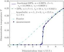
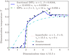
for experiment I, and

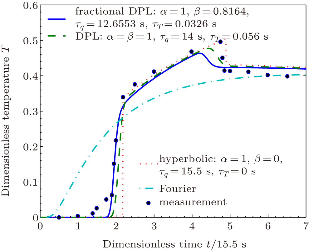
for experiment III. The results of the parameter estimation in this study for the fractional DPL model, together with the previous non-Fourier models of Refs. [8] and [9], are summarized in Table 1. A comparison between the measured and the estimated temperatures for experiment I is shown in Fig. 1. It can be seen that the fractional DPL prediction (solid line) closely follows the measurement and captures the rapid increase in the temperature well. For experiment III, the comparison of the measured and the estimated temperatures are shown in Fig. 2. Although there are still differences with the experimental data, the calculation shows that the L2 error of the fractional DPL model for experiment III is the lowest in the three models. The fractional DPL model also well predicts the rapid increase in the measured temperature. However, the decrease is significantly less rapid than that of the measurement, like the DPL model. The above comparison shows that the fractional DPL model can give a good temperature prediction for the problem under study. Thus, the fractional DPL model in this paper provides a new theoretical perspective for an in-depth study of non-Fourier heat conduction.
| Table 1. Comparison of different non-Fourier heat equations in modelling experiments I and III.[8] |
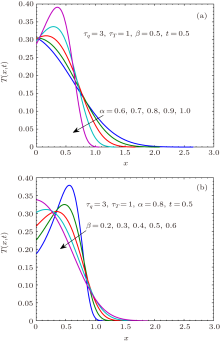
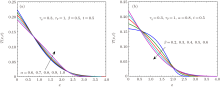
In order to show the behavior of the solution to the system (13)– (16), several numerical examples are also given for the initial condition g(x) = δ (x), where δ is the Dirac distribution. Generally, we assume τ q > τ T in the DPL model. While a large number of applications of the DPL model are specifically related to the case τ q < τ T, such as the ultrafast pulse-laser heating on a metal film, [3, 4] we also make a comparison for τ q > τ T and τ q < τ T using Figs. 3– 5. Figures 3 and 4 show the temperatures for various α and β when τ q > τ T and τ q < τ T, respectively. It can be observed that figure 3 displays the wave character and figure 4 displays the diffusive character of the temperature. Figure 5 shows the solution T for fixed positions. It shows that the ratio τ q/τ T affects the time at which the temperature of a fixed position reaches the maximum.
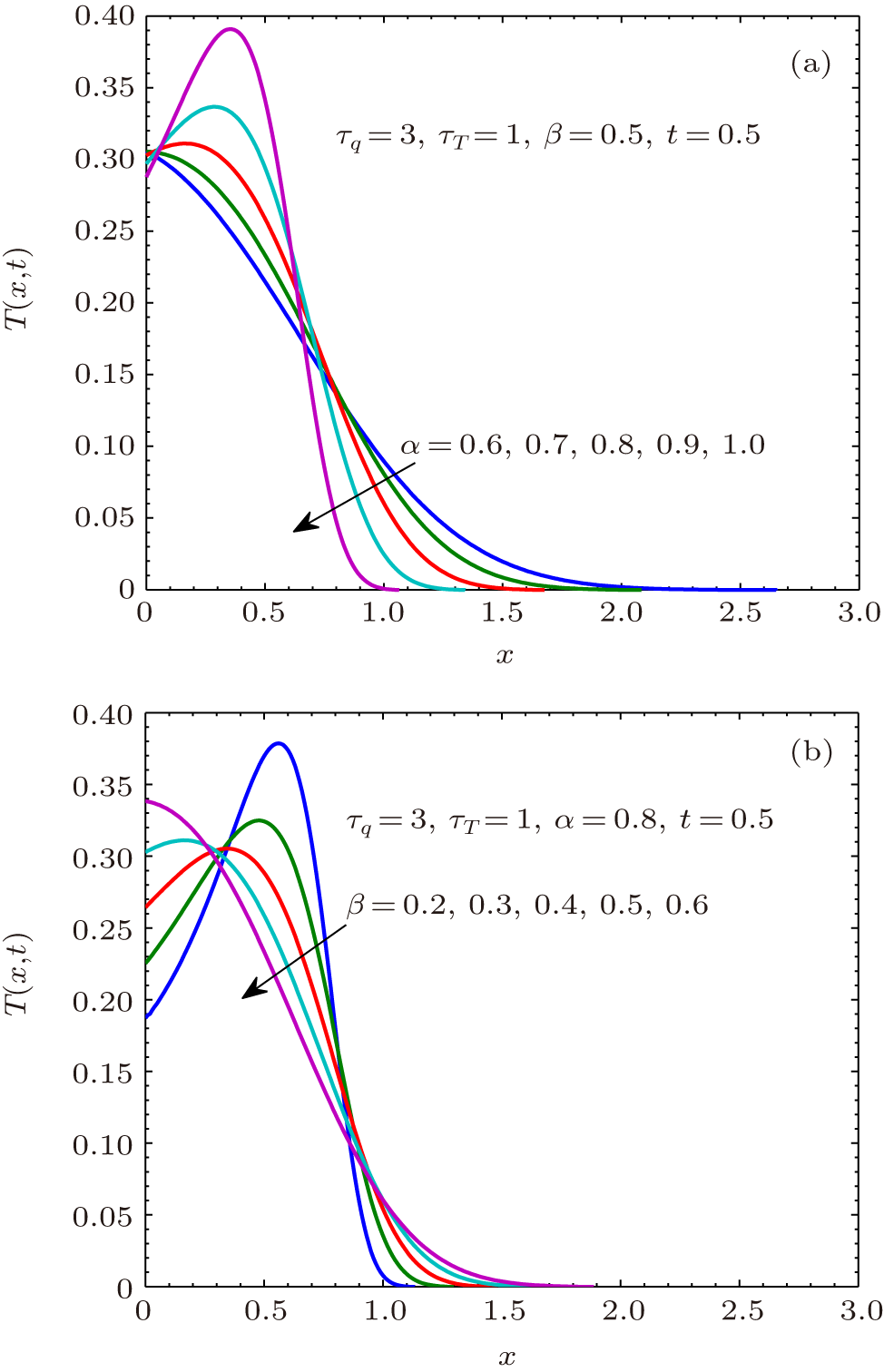 | Fig. 3. Plots of T(x, t) for T(x, 0) = δ (t) when τ q > τ T. The arrow indicates plots with increasing (a) α or (b) β . |
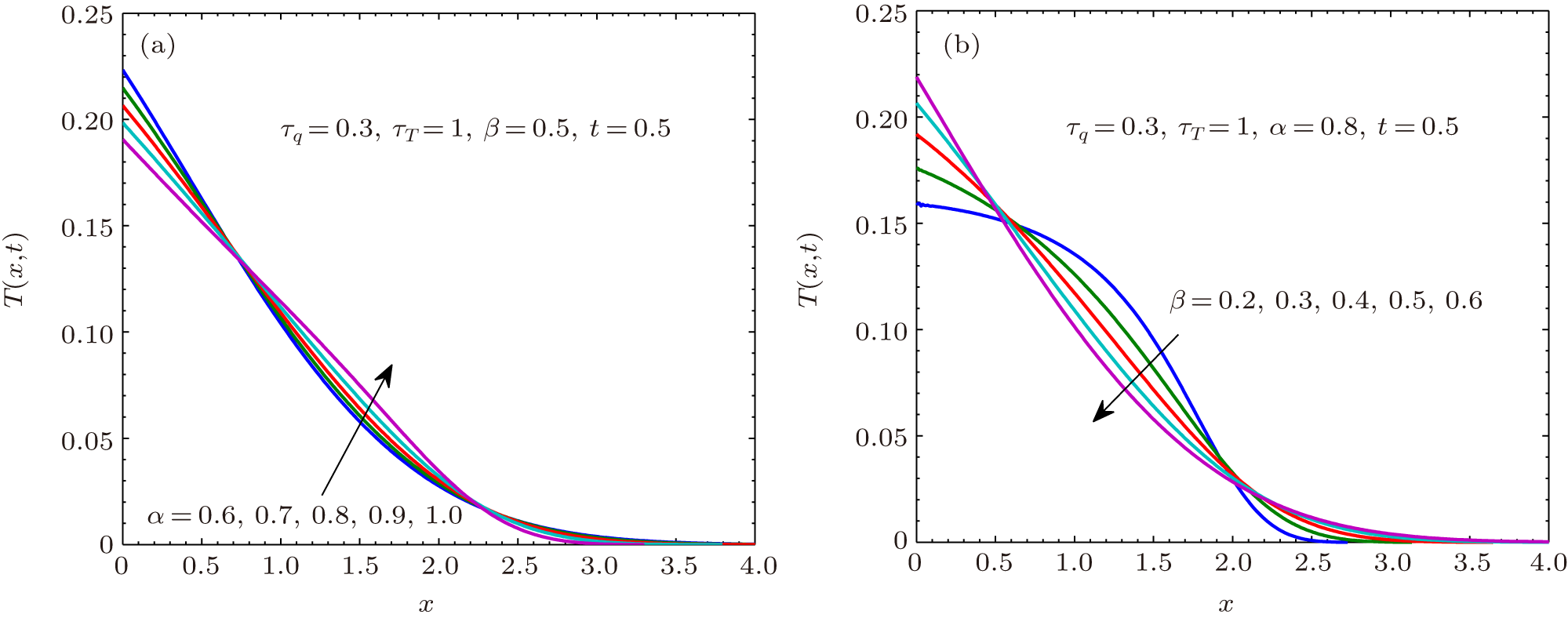 | Fig. 4. Plots of T(x, t) for T(x, 0) = δ (t) when τ q < τ T. The arrow indicates plots with increasing (a) α or (b) β . |
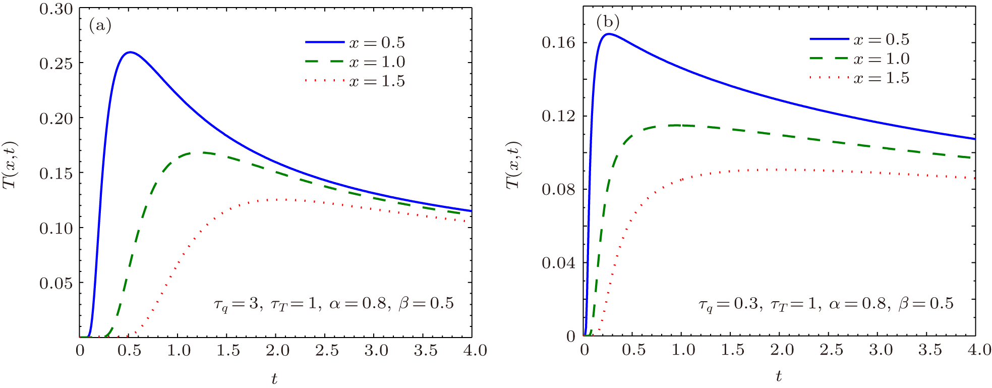 | Fig. 5. Plots of T(x, t) for T(x, 0) = δ (t) when the positions are considered: (a) τ q = 3, (b) τ q = 0.3. |
In the present paper, we study the time fractional DPL model for bioheat transfer. Based on the experiments of Mitra et al., [8] the exact solution of the fractional DPL heat conduction equation is obtained under suitable initial and boundary conditions with the help of integral transforms and the H-function. The model is further used to study the temperatures of experiments I and III in Ref. [8] with the nonlinear least-square method and a consistent result is obtained. This shows that the fractional DPL model can help to promote the understanding of heat conduction in biological tissues, such as human tissue. The effect of the model parameters are also discussed. The wave and the diffusion characters are shown. We hope that the fractional DPL heat conduction model will be useful in the description of non-Fourier heat conduction.
| 1 |
|
| 2 |
|
| 3 |
|
| 4 |
|
| 5 |
|
| 6 |
|
| 7 |
|
| 8 |
|
| 9 |
|
| 10 |
|
| 11 |
|
| 12 |
|
| 13 |
|
| 14 |
|
| 15 |
|
| 16 |
|
| 17 |
|
| 18 |
|
| 19 |
|
| 20 |
|
| 21 |
|
| 22 |
|
| 23 |
|
| 24 |
|
| 25 |
|
| 26 |
|
| 27 |
|
| 28 |
|
| 29 |
|
| 30 |
|
| 31 |
|
| 32 |
|
| 33 |
|
| 34 |
|
| 35 |
|
| 36 |
|
| 37 |
|
| 38 |
|
| 39 |
|
| 40 |
|
| 41 |
|
| 42 |
|
| 43 |
|
| 44 |
|
| 45 |
|
| 46 |
|
| 47 |
|
| 48 |
|
| 49 |
|
| 50 |
|