
Observer of a class of chaotic systems: An application to Hindmarsh–Rose neuronal model*
[Luo Run-Zi† , Zhang Chun-Hua]
, Zhang Chun-Hua]
|
|


†Corresponding author. E-mail: luo rz@163.com
*Project supported by the National Natural Science Foundation of China (Grant Nos. 11361043 and 61304161), the Natural Science Foundation of Jiangxi Province, China (Grant No. 20122BAB201005), and the Scientific and Technological Project Foundation of Jiangxi Province Education Office, China (Grant No. GJJ14156).
This paper first investigates the observer of a class of chaotic systems, and then discusses the synchronization between two identical Hindmarsh–Rose (HR) neuronal chaotic systems. Both the drive and response systems are assumed to have only one state variable available. By constructing proper observers, some novel criteria for synchronization are proposed via a scalar input. Numerical simulations are given to demonstrate the efficiency of the proposed approach.
Chaos is a very interesting nonlinear phenomenon. Since the synchronization between two identical chaotic systems with different initial conditions has been proposed by Pecora and Carroll in 1990, [1] chaos synchronization has received increasing attention due to its potential applications in many areas, such as secure communication, information processing, biological systems, and chemical reaction. Many methods have been proposed for chaos synchronization, including the feedback method, [2] back-stepping technique, [3]H∞ approach, [4] sliding control, [5] and so on.
In general, there are two types of the drive-response synchronization framework. In the first, which is called chaos-based synchronization, [6, 7] the drive system and response system are all chaotic systems. The second is the so called observer-based synchronization in which the drive system is a chaotic system and the response system is an observer of the drive system.
There are many results about the chaos-based synchronization in the literature.[8– 14] However, most of the existing literature concerning the chaos-based synchronization problem needs several controllers to realize synchronization. From the view point of practical applications, it is well known that the controllers to realize synchronization must be simple, efficient, and easy to implement. The fewer the number of the designed controllers, the better the synchronization method. Thus, it is desired to design a scalar controller to synchronize chaotic systems. Many efforts have been devoted to synchronize chaotic systems by using only one scalar controller. For example, a systematic design procedure to synchronize a class of chaotic system in a so-called strict feedback form based on back-stepping procedure was presented in Ref. [15]. This approach needs only a single controller to realize synchronization, no matter how many dimensions the chaotic system contains. In Ref. [16], the author investigated the stabilization and synchronization of Genesio– Tesi system via single variable feedback controller. Based on the adaptive sliding mode control strategy, the synchronization of a Chen hyper-chaotic system with noise-perturbed via a single control signal was discussed in Ref. [17]. The synchronization of a class of three-dimensional fractional-order chaotic systems was investigated in Ref. [18]. Based on the Lyapunov stability theory and adaptive control technique, a single adaptive-feedback controller was developed to synchronize a class of fractional-order chaotic systems. Some simple and easily verified criteria for the stabilization of impulsive dynamical networks under a single impulsive controller and/or a single negative state-feedback control were given in Ref. [19].
It should be noted that the schemes proposed in Refs. [15]– [19] were under the condition that the states of the drive system and the response system were completely known. It is well known that the states both in the drive and response systems are partially or fully unavailable in many practical control problems.
Motivated by the above discussion, this paper discusses the synchronization between two identical Hindmarsh– Rose (HR) neuronal chaotic systems. Both the drive and response systems are assumed to have only one state variable available. By constructing proper observers, some novel criteria for synchronization are proposed via a scalar input. Numerical simulations are given to demonstrate the efficiency of the proposed approach.
The layout of the rest of this paper is organized as follows. The design of the observer of a class of chaotic systems is introduced in Section 2. Section 3 investigates the synchronization scheme between two identical HR neuronal chaotic systems. Section 4 includes several numerical examples to demonstrate the effectiveness of the proposed approach. Finally, some conclusions are given in Section 5.
It is well known that not all of the state variables are available for some chaotic systems. For example, in some systems only the output is available and the output may be a state variable. However, in the control or synchronization of chaotic systems most of the controllers are designed by using all of the systems' state variables. In this paper we assume that both the drive and response systems have only one state variable available. In order to construct a suitable controller we use the estimated values instead of the unavailable variables. Thus, the unavailable variables must be estimated when designing the proper controller. For this end in this section we consider the observer of the following chaotic system:

where x = (x1, x2, x3)T ∈ R3× 1 is the state vector of system (1), f(x1), g(x1), h(x1) are functions of x1, a ≠ , c3> 0 and bi (i = 1, … , 8), c1, c2 are the system's parameters which are known in advance.
Suppose that the available state variables of system (1) is x1, the purpose of this section is to design a suitable observer such that the other state variables x2 and x3 of system (1) can be recovered. For this end, we introduce the following system:
where 

Remark 1 Reference [20] considered the observer of the following class of chaotic system:
Obviously, system (3) is a special case of system (1). Many chaotic systems, which do not belong to system (3), can be written as in the form of Eq. (1), such as the Rö ssler system[21] and the Hindmarsh– Rose neuron system.[22] In addition, the method used in designing system (2) is different from that of observer (3) or (5) in Ref. [20]. The main difference is that in system (2) we have introduced a constant k> 0, , which is the key point in proving the stability of the error system (5).
Prior to going any further, we make the following assumption.
Assumption 1 There exists a non-negative constant M such that 
By taking
one can obtain the following theorem.
Theorem 1 If k is chosen as inequality (4), then system (2) is an observer of system (1).
Proof Let us define 
thus we obtain the error dynamic system as follows:

For system (5) we can prove that

In fact, we choose the Lyapunov candidate as

Its derivative along the trajectories of system (5) is
By combining using a2+ b2≥ 2|ab| and inequality (4), one obtains
Based on the Lyapunov stability theory, the error system (5) is globally stable about the origin. Therefore, we have

which implies that 

In this section, we take the HR neuronal model as an example to show the application of observer (2) in synchronization.
The HR neuronal model was first proposed by Hindmarsh and Rose as a mathematical representation of the firing behavior of neurons.[22] The form of HR system is given by

where z1 represents the membrane potential, z2 is the recovery variable associated with the fast current of Na+ or K+ ions, and z3 is associated with the slow current of Ca+ ions. a, b, c, d, r, s, k, Iext are real constants. If the parameters are chosen as a = 3.0, b = 1.0, c = 1.0, d = 5.0, r = 0.006, s = 4.0, k = 1.6, then regular bursting can be observed for Iext = 2.0 and chaotic bursting can be obtained for Iext = 3.0, respectively (see Fig. 1). Since when r = 0.006 system (6) is chaotic, in the following we assume r> 0.
 | Fig. 1. Time series of system (6) with z1 = 0.1, z2 = 0.2, z3 = 0.3: (a) regular bursting Iext = 2.0, (b) chaotic bursting Iext = 3.0. |
It is easy to see that system (6) is not of the form as in Eq. (1). However, it can be transformed into system (1) after some simple state transformation. For example, if we let z1 = x2, z2 = x3, z3 = x1, then equation (6) can be rewritten as
where p = rs, q = rsk. Obviously, system (7) is in the form of system (1).
Assume that the available states of system (7) is x1, in order to synchronize system (7), we should to estimate x2 and x3. Based on system (2), we obtain the following observer:
where 

Suppose that system (7) is the drive system, then the response system is
where u is the controller. If the available state of system (9) is y1, then u is the function of x1, y1. Without loss of generality, we can assume that u = u(x1, 


For the end of estimating y2 and y3, we give the following observer for system (9):
By defining e1 = y1– x1, e2 = y2– x2, e3 = y3– x3 and from Eqs. (7) and (9), one obtains
Remark 2 The constant k in systems (8) and (10) is designed as inequality (4).
Before presenting our other main result, we introduce a Lemma and an assumption which will be used in our proofs.
Lemma 1[20] If 

is globally asymptotically stable, where λ > 0.
Assumption 2 There exists a non-negative constant M such that |yi| ≤ M, |ŷ 2| ≤ M, |ŷ 3| ≤ M, i = 1, 2, 3. We take

and

The following Theorem 2 ensures that systems (7) and (9) can reach synchronization.
Theorem 2 If the observer of systems (7) and (9) are, respectively, selected as systems (8) and (10), and the controllers u and constant l are, respectively, chosen as Eq. (13) and inequality (14), then synchronization between systems (7) and (9) can be achieved.
Proof Choose the following Lyapunov function:

The derivative of the above function along the trajectories of system (11) is

where e2y = ŷ 2– y2 and
In view of inequality (14), one can easily know that the three principal minor determinants of Q are greater than 0, which implies that Q is a positive definite matrix. Thus the three eigenvalues of Q are also greater than 0. Without loss of generality, we assume that λ is the minimal one.
From inequality (15), one obtains

Keep in mind that 

Remark 3 There are two ways to get l. (i) We can first estimate M by simulation and then calculate l via inequality (14). (ii) We can obtain l by using adaptive method. For example, if we choose 
The numerical simulations demonstrating and verifying the proposed control methods are presented in this section. The parameters of HR neuron are chosen as a = 3.0, b = 1.0, c = 1.0, d = 5.0, r = 0.006, s = 4.0, k = 1.6, and Iext = 3.0, so that HR neuron shows chaotic phenomenon.
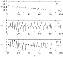
The constants k and l are taken as k = l = – 200. The initial conditions of the drive system (7) and response system (9) are set as (x1(0), x2(0), x3(0)) = (0.1, 0.2, 0.3) and (y1(0), x2(0), x3(0)) = (0.6, 0.7, 0.8), respectively. Without applying any control, synchronization of the two HR neurons (7) and (9) cannot be achieved, as shown in Fig. 2. The initial conditions of the two observers (8) and (10) are chosen as (

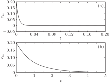
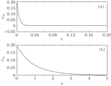
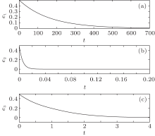
Figure 3 shows the time evolution curves between drive system (7) and observer (8). Figure 4 displays the time evolution curves between response system (9) and observer (10). The synchronization errors between drive system (7) and response system (9) are shown in Fig. 5. It is obvious that the synchronization errors converge asymptotically to zero and two HR neurons systems are indeed achieved synchronization when only one controller is used.
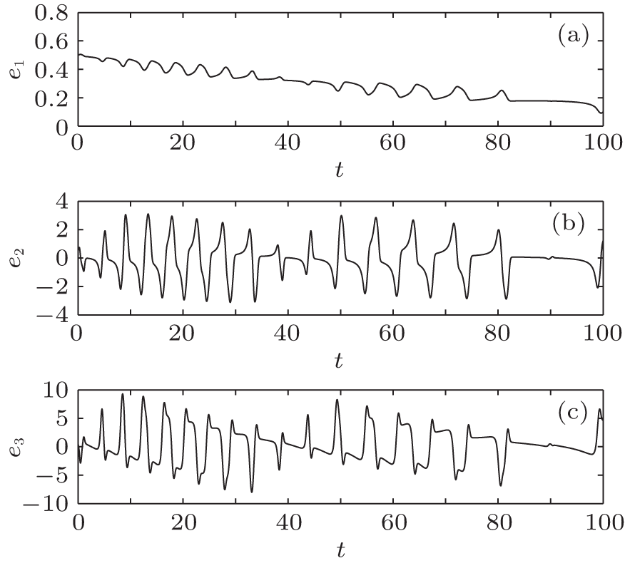 | Fig. 2. Synchronization errors of the HR systems (7) and (9) without control. (a) e1, (b) e2, (c) e3. |
 | Fig. 3. The time evolution of errors e2x (a) and e3x (b) between drive system (7) and observer (8). |
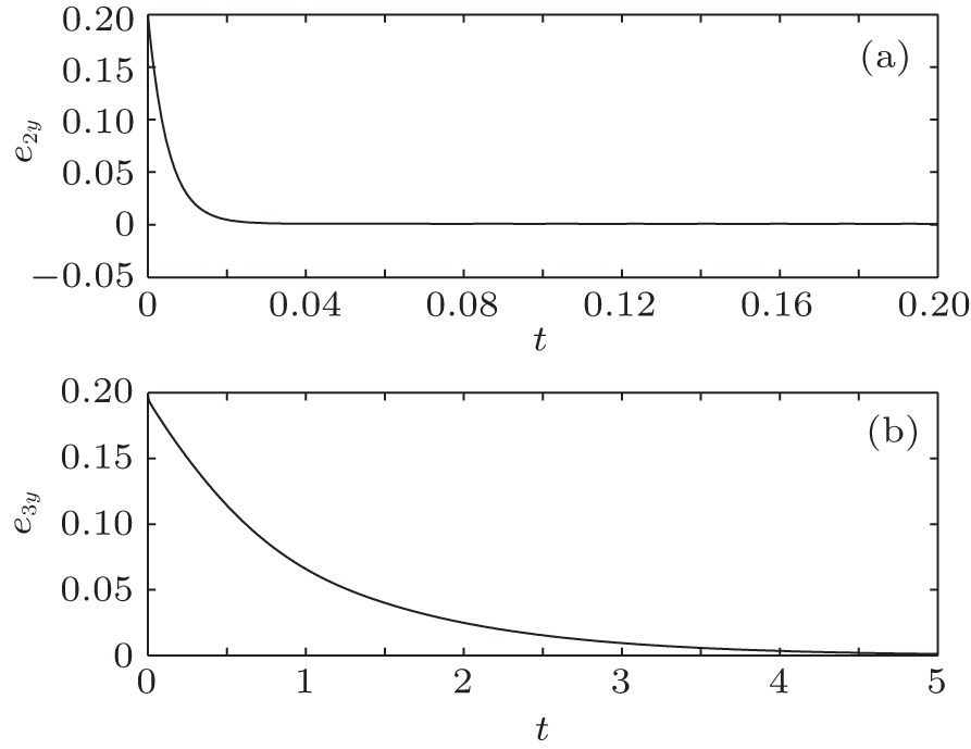 | Fig. 4. The time evolution of errors e2y (a) and e3y (b) between response system (9) and observer (10). |
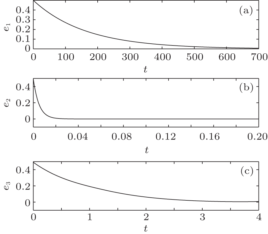 | Fig. 5. Synchronization errors of the HR systems (7) and (9) with control u = -l(ŷ 2- |
Remark 4 It is easy to see that in this paper we have made four chaotic systems synchronize with each other, they are: drive system (7), response system (9), observe systems (8) and (10).
This work investigates the observer of a class of chaotic systems with only one state variable available. Based on the observers designed for the drive and response systems, some new sufficient conditions are presented for achieving synchronization between two identical HR neuronal chaotic systems. In our control scheme we do not need to use the unavailable states of the drive and response systems, thus our approach is more realistic and practical than most of the existing methods since they have assumed that all of the states are available. Finally, numerical simulations are carried out to verify the efficiency of the proposed controller.
| 1 |
|
| 2 |
|
| 3 |
|
| 4 |
|
| 5 |
|
| 6 |
|
| 7 |
|
| 8 |
|
| 9 |
|
| 10 |
|
| 11 |
|
| 12 |
|
| 13 |
|
| 14 |
|
| 15 |
|
| 16 |
|
| 17 |
|
| 18 |
|
| 19 |
|
| 20 |
|
| 21 |
|
| 22 |
|