


Bifurcation behavior and coexisting motions in a time-delayed power system*
[Ma Mei-Ling, Min Fu-Hong† ]
]
]
|
|


†Corresponding author. E-mail: minfuhong@njnu.edu.cn
*Project supported by the National Natural Science Foundation of China (Grant Nos. 51475246 and 51075215), the Natural Science Foundation of Jiangsu Province of China (Grant No. Bk20131402), and the Scientific Research Foundation for the Returned Overseas Chinese Scholars, State Education Ministry of China (Grand No. [2012]1707).
With the increase of system scale, time delays have become unavoidable in nonlinear power systems, which add the complexity of system dynamics and induce chaotic oscillation and even voltage collapse events. In this paper, coexisting phenomenon in a fourth-order time-delayed power system is investigated for the first time with different initial conditions. With the mechanical power, generator damping factor, exciter gain, and time delay varying, the specific characteristic of the time-delayed system, including a discontinuous “jump” bifurcation behavior is analyzed by bifurcation diagrams, phase portraits, Poincaré maps, and power spectrums. Moreover, the coexistence of two different periodic orbits and chaotic attractors with periodic orbits are observed in the power system, respectively. The production condition and existent domain of the coexistence phenomenon are helpful to avoid undesirable behavior in time-delayed power systems.
A power system is essentially a multivariable dynamic system with strong nonlinear characteristics. With the development of large-scale interconnected power systems, the complexity of operations in a power system has increased.[1, 2] Chaotic oscillation is a nonlinear phenomenon which indeed exists in the power system, which will lose stabilization, even collapse events in succession and incur a huge amount of economic loss.[3] Recently, the nonlinear phenomenon in power systems has received significant attention in the literature. The earlier work mainly focused on the dynamic instability, [4– 7] bifurcation behavior, [8– 13] and the methods to mitigate the chaotic electromechanical oscillation.[14– 18]
Time delay is unavoidable which exists widely in the measurement and control loops of power systems. In the past, the feedback controllers were designed through the local information, so time delays in power systems were ignored with little error.[20] However, power systems become larger and more complicated in modern times, where generators are connected by systematic tie lines over a long distance and the exciter inputs are taken from remote buses. Under these conditions, the time delay can vary from tens to several hundred milliseconds or more which may lead to unacceptable performance, such as loss of synchronism and instability in power system.[13] Jia[21] analyzed the impact of time delay on a fourth-order dynamic power system[10] for the first time and found time delays have a destabilizing impact. Furthermore, the maximum time delay which can sustain without losing small signal stability was estimated in power systems and the stability region was also traced by an optimal-based algorithm.[22, 23] However, the influence of the other parameters on the time-delayed system has not been discussed in the related literature. More works were devoted to the investigation of time delays in power systems. Ayasun[24] presented a direct method to compute the delay margin of power systems with single and commensurate time delays. Similarly, Federico[25] gave a relative simple method to define the small-signal stability of the delay differential algebraic equations. Liu[26] studied the effect of signal time delay in the wide area measurement system on power system stability. Chowdhury[27] found that time delay does not influence the equilibrium structure, but has an impact on the stability properties. Though the influence of time delay on the small signal stability region of power systems has been studied, the bifurcation behavior and chaotic attractors of the time-delayed power system have seldom investigated.
Multistability is a special characteristic which has commonly been found in nonlinear dynamic systems, which increases the complexity and unpredictability of systems. For a given set of parameters, multistable systems have the ability to exhibit a number of coexisting motions. The initial condition decides intensively the final states of chaotic attractor and periodic orbits.[28] Recently, there have been lots of researches on the coexisting motions of physical, chemical and biological systems, [28– 34] but the study in power systems has seldom been investigated. Vaithianathan[19] has reported firstly the occurrence of a phenomenon when four different strange attractors, i.e., a stable equilibrium, a stable limit cycle and two strange attractors coexist in a power system. No more further study on coexistence in power systems has been found.
The purpose of this paper is to study the multistability of power systems. The coexistence phenomenon in a fourth-order time-delayed power system is studied for the first time. Much coexisting motions generated by different initial conditions are demonstrated in the same basin. Together with the bifurcation diagrams, phase portraits, Poincaré maps, and power spectrums, two coexisting modes are concluded to illustrate the rare behavior. The domain of coexistence in time-delayed power system is also given respectively.
The single-machine-infinite-bus system, as shown in Fig. 1, considers the excitation model which provides direct current for generator excitation windings to form the air gap magnetic field. Similar to the second-order power system, [35] the angle dynamics can be represented as the following equations:
where δ is the generator angle, ω is the machine frequency, E′ is the generator voltage behind the transient reactance, H is the moment of inertia in second, D is the generator damping factor, V0 is the infinite bus voltage, x represents the transmission line reactance and 

where 
and Efd is the exciter output voltage with
where Efdr is the input signal of the wind-up limiter which limits the excitation voltage Efd to be strictly from Efdmin to Efdmax.
 | Fig. 1. The single-machine-infinite-bus system. |
To simplify the equation, equation (2) can be rewritten as

The excitation field control is simply presented by the transfer function in Fig. 1, and then we have

where Vref is the reference bus voltage, TA is the time constant, KA is exciter gain, and Efd0 is the reference voltage. The bus voltage at the generator bus terminal is given by

From the above equations, the fourth-order power system is described as

The dissipation of the power system is derived as follows:

Since H,
Time delay always exists widely in nonlinear power systems. Jia first investigated the impact of time delay on power system small signal stability.[21] Due to the long distance transmission, time delay is mainly found in the exciter model and influences the voltage V at the bus terminal. Assume that there is a time delay τ in the measurement of V, and then the equation (8) can be rewritten as
where

Previous studies on the single-machine-infinite-bus system have mainly focused on the stability region while the dynamics analysis of the system has seldom been studied. In the following, abundant chaotic and periodic attractors will be demonstrated through phase portraits and sequence diagrams. The system parameters are chosen in per unit f0 = 60, V0 = 1, Vref = 1.05, Efdmax = 5, Efd0 = 2, Efdmin = 0,
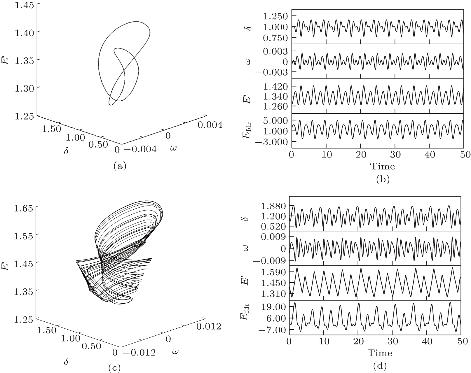 | Fig. 2. Typical attractors of the system. (a) and (b) Periodic phase portrait and sequence diagram for Pm = 1.233, D= 2, KA= 150, τ = 0.068, (c) and (d) chaotic phase portrait and sequence diagram for Pm = 1.35, D= 2, KA= 150, τ = 0.068. |
Due to the different initial conditions, the coexisting motions in nonlinear systems usually appear with the same parameter values, which are the significant characteristics of multistable systems, such as weakly dissipative systems, coupled systems, and timed-delay systems.[32] The time-delayed power system in Eq. (10) will produce abundant coexisting behavior with different initial conditions, which may be trapped into the sustained chaotic oscillation after a large disturbance. The irregular oscillation will even result in a power system accident or large area power blackout. To better understand the complex dynamics of the system and explore more coexisting regions, the typical bifurcation diagrams for mechanical power Pm, generator damping factor D, exciter gain KA, and time delay τ are investigated in this section. For the diverse initial conditions, multiple regions of coexistence will be encountered in a time-delayed power system. In the following simulation, the initial condition 1, IC1 = (0.9857, − 0.0004, 1.4046, 2.3282), and initial condition 2, IC2 = (1.4377, 0.0032, 1.3389, 10.9338), are chosen respectively.
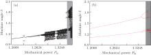
The mechanical power Pm determines the speed of the generator and has a great influence on stable operation in the power system. The bifurcation diagrams for Pm with IC1 and IC2 are shown in Figs. 3(a) and 3(b) respectively, in which Pm is varied in the range of [1.2, 1.356] and the other system parameters are used with D= 2, KA= 150, and τ = 0.068. From Figs. 3(a) and 3(b), it is easy to find that the two bifurcation diagrams are quietly different in the region Pm ∈ [1.2, 1.34] and then begin to merge together at Pm = 1.34. The two diagrams are the same and show the route of period-doubling bifurcation to chaos in the gray areas.
 | Fig. 3. Bifurcation diagrams for mechanical power Pm with different initial conditions, (a) IC1 and (b) IC2. |
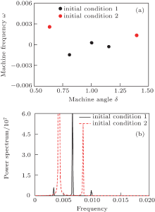
From Fig. 3(a), a sudden “ jump” phenomenon which can only be found in discontinuous systems[28] is observed in the interval Pm ∈ [1.22989, 1.23455]. The bifurcation breaks into pieces and changes from one line to three short ones and then back to one. Correspondingly, the phase portrait with IC1 changes from period-1 to period-3, and then becomes the period-1 motion, which this “ jump” phenomenon cannot be observed in Fig. 3(b). The bifurcation diagram with IC2 presents two lines in the same interval, which shows the period-2 phase portraits. Due to the difference of the two bifurcation diagrams, the coexistences of period-3 and period-2 orbits can be exhibited here. In Fig. 4, the phase portraits of the coexisting motions at Pm = 1.233 are displayed in six planes as δ – ω , δ – E′ , δ – Efdr, ω – E′ , ω – Efdr, and E′ – Efdr from a different perspective. Additionally, poincaré maps and power spectrums are adopted to prove the correctness, as shown in Fig. 5. The black dots represent the attractors with IC1 and the red dots denote the attractors with IC2. There are three black dots and two red dots in Fig. 5(a), and three black peaks and two red peaks in Fig. 5(b), which totally match the period-3 and period-2 attractors.
 | Fig. 4. The phase portrait of coexistence of period-3 and period-2 orbits. (a) δ – ω , (b) δ – E′ , (c) δ – Efdr, (d) ω – E′ , (e) ω – Efdr, and (f) E′ – Efdr. |
 | Fig. 5. Poincaré maps and power spectrums of the coexistence of period-3 and period-2 orbits, (a) poincaré maps, (b) power spectrums. |
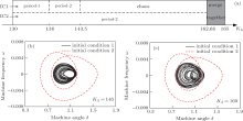
From the two bifurcation diagrams with different initial conditions in Fig. 3, diverse types of coexisting motions can be found. The specific coexisting regions are shown in detail in Fig. 6(a). The motion of the system with IC1 changes from period-1 to period-3 orbit immediately at mechanical power Pm = 1.2299. With the parameter Pm varying, the motion in the power system experiences period-1 and period-2 orbits in turn until Pm increases to 1.274, and then the system becomes chaotic motion. Among the range of chaotic motion, there is a small periodic motion of multiple periods in range of [1.3228, 1.319]. Moreover, the system with IC2 becomes much simpler which only has period-2 and period-4 orbits before Pm = 1.341. After that, the trajectories with IC1 and IC2 will keep the same and the coexistence disappears. To better visualize the dynamics of the coexistence, a period-8 motion coexists with a period-2 orbit at Pm = 1.314, and a chaotic attractor coexists with a period-4 orbit at Pm = 1.338 are shown in Figs. 6(b) and 6(c), respectively.
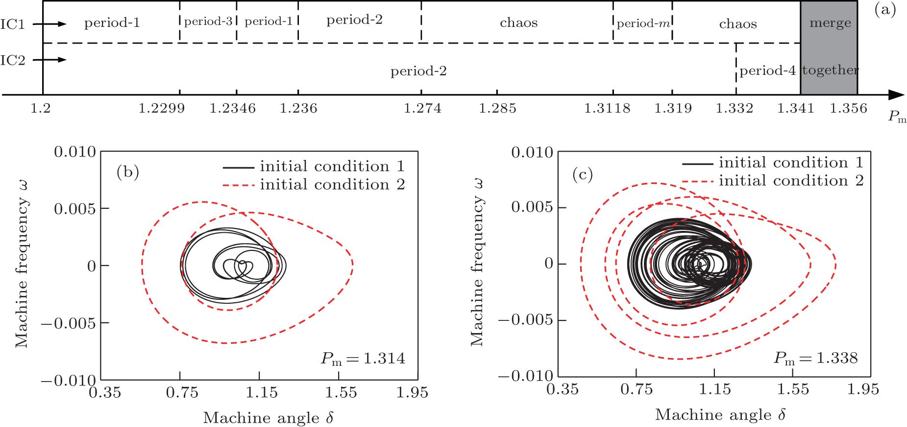 | Fig. 6. (a) Parameter domains of coexisting motions as Pm varies (“ m” is multiple). Coexistence with different motions, (b) period-8 and period-2, (c) chaos and period-4. |
The damping factor D is a comprehensive damping coefficient which relates to the real speed of generator. Here, the system parameters are given by Pm = 1.3, KA= 150, τ = 0.068. The bifurcation diagrams for D with IC1 and IC2 are shown in Fig. 7, which indicates that the system behaves periodically in a rather larger range, while chaotic attractors only take place in small regions. In Fig. 7(a), the system with IC1 behaves chaotically in the region D ∈ [1.28, 2.42]. However, the chaotic region is in D ∈ [0, 1.12] with IC2, as shown in Fig. 7(b). In the rest of the parameters range, the system with IC1 and IC2 will have periodic motion all the time. With the damping factor D increasing, the two bifurcation diagrams coincide with each other to behave periodically from D= 13.6, and the coexisting phenomenon in the power system will disappear.
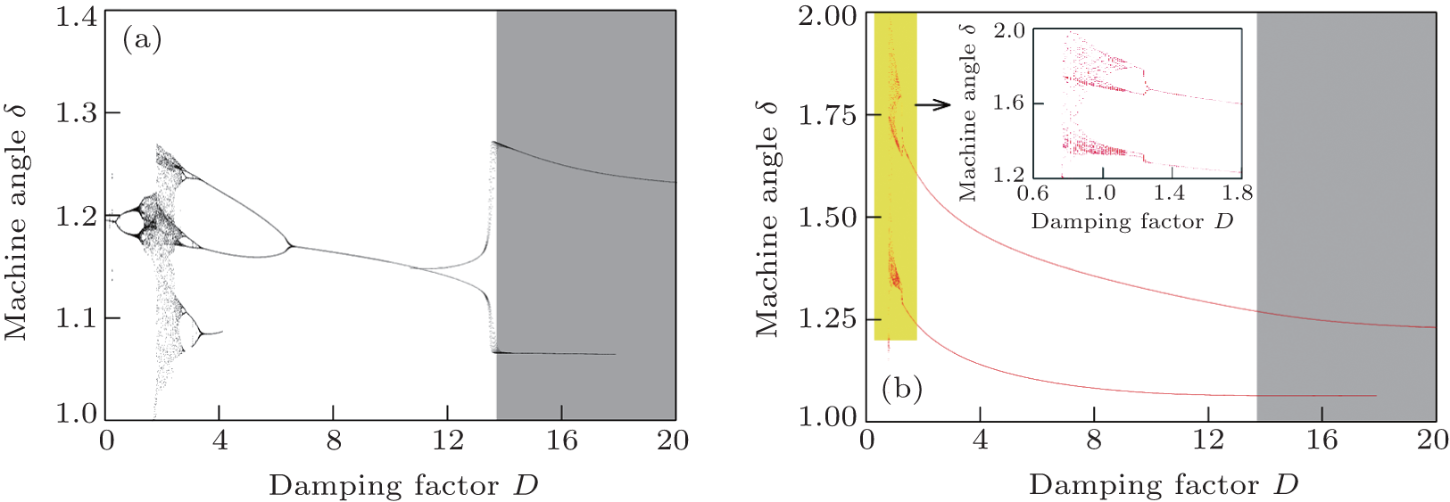 | Fig. 7. Bifurcations for the damping factor D with different conditions. (a) IC1 and (b) IC2. |
Due to the peculiar characteristics, a lot of coexisting motions can be observed in range of D ∈ [0, 13.6]. The specific coexisting domains are also displayed in Fig. 8(a) in detail. The time-delayed power system with IC1 experiences period-1 and period-2 before D= 1.28, while the system with IC2 undergoes instability region, chaos, and periodic motions. Therefore, the abundant coexisting phenomenon can be found in this region, such as the coexisting motions of period-2 orbit with chaos at D= 0.84 in Fig. 8(b), and period-2 with period-4 orbit at D= 1.12 in Fig. 8(c). When the damping factor D increases to 1.28, the system with IC1 goes through chaos, period-m (periodical motion with multiple periods), period-3, period-2, period-1 orbits and then back to period-2 orbit. However, the system displays only one stable state of period-2 with IC2. Hence, in this interval, there are many attractors coexisting with period-2, such as the coexistence of period-4 with period-2 motions at D= 2.93 in Fig. 8(d), and period-1 with period-2 motions at D= 8 in Fig. 8(e).
 | Fig. 8. (a) Parameter domains of coexisting motions with D varying (“ m” is multiple). Coexisting motions with different conditions. (b) Period-2 and chaos, (c) period-2 and period-4, (d) period-4 and period-2, (e) period-1 and period-2. |
The exciter gain KA of the excitation model in power system determines the stability of the generator. In this section, the system parameters Pm = 1.3, D= 2, and τ = 0.068 are fixed, and the exciter gain KA is varied from 130 to 162.66. The bifurcation diagrams with KA varying are shown in Fig. 9. Compared with Figs. 3 and 7, the diagrams in Fig. 9 are the simplest, and especially in Fig. 9(b) only two straight lines exhibit, which mean the system with IC2 will display period-2 attractors all the time. When the exciter gain KA increases to KA= 162.66, the bifurcation diagram with IC1 in Fig. 9(a) also becomes the two straight lines. The exact coexisting regions are also given in Fig. 10(a). Three types of coexisting phenomena can be obtained in the range of KA ∈ (130, 162.66), including the coexistence of period-1 with period-2 motion, and different period-2 motions, chaos and period-2 motion. The two bifurcation diagrams with different conditions are the same in the region [162.66, 165]. Moreover, in different parameter regions, the structures of the coexistence of chaotic and period-2 orbits are different. As seen in Fig. 10, the two coexisting motions for KA= 146 and KA= 160 have the same coexistence regions with different structures, respectively.
 | Fig. 9. Bifurcations for the exciter gain KA with different initial conditions. (a) IC1 and (b) IC2. |
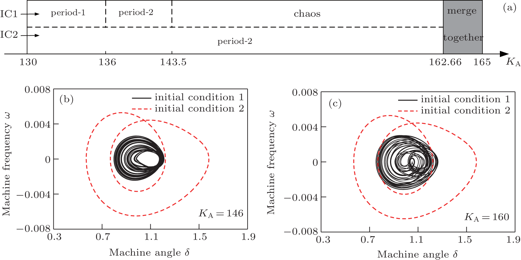 | Fig. 10. (a) Parameter domains of coexisting motions with KA varying. Coexisting motions of chaos and period-2 orbit. (b) KA = 146, (c) KA = 160. |
Time delay is unavoidable in nonlinear power systems. The delay margin of system (10) is already calculated in Refs. [22]– [24], and it only provides the maximum time delay which the power system can sustain. However, how the time delay influences the characteristics of the system is not shown in Refs. [22]– [24]. Here, the bifurcation for time delay τ is given in the range of [0, 0.1] with Pm = 1.3, D = 2, and KA = 150, and the different coexisting motions are also obtained. In Fig. 11, two bifurcation diagrams for time delay τ with IC1 and IC2 merge together in τ ∈ [0, 0.0156) ∪ (0.085, 0.1]. Similar to the “ jump” phenomenon in the bifurcation for Pm in Fig. 3(a), a sharp decrease is also observed for the upper curve at τ = 0.0156 in Fig. 11(a), and the curve converges gradually toward the lower curve. The chaotic motions are also shown in a small range of τ ∈ [0.065, 0.075]. Two simple inclined lines for the case with IC2 are presented in Fig. 11(b), which indicates the system has periodic motions. Moreover, a periodic-doubling in Fig. 11(b) occurs in the region τ ∈ [0.02, 0.03], and period-4 orbits can be observed. From the bifurcation in Fig. 11, the parameter domains of coexistence with time delay τ varying are carried out in Fig. 12(a). There are at least eight types of coexisting phenomenon in the region τ ∈ [0.0156, 0.0853]. The system goes through period-2, period-1, period-2, chaos, period-m, period-3, and period-2 motions in turn for IC1, while there are only period-2 and period-4 motions with IC2. To confirm the occurrence of the coexistence, the typical coexisting motions are exhibited as shown in Fig. 12, such as period-1 with period-4 orbits at τ = 0.025 in Fig. 12(a), and period-4 with period-2 orbits at τ = 0.076 in Fig. 12(b).
 | Fig. 11. Bifurcations for time delay τ with different initial conditions, (a) IC1 and (b) IC2. |
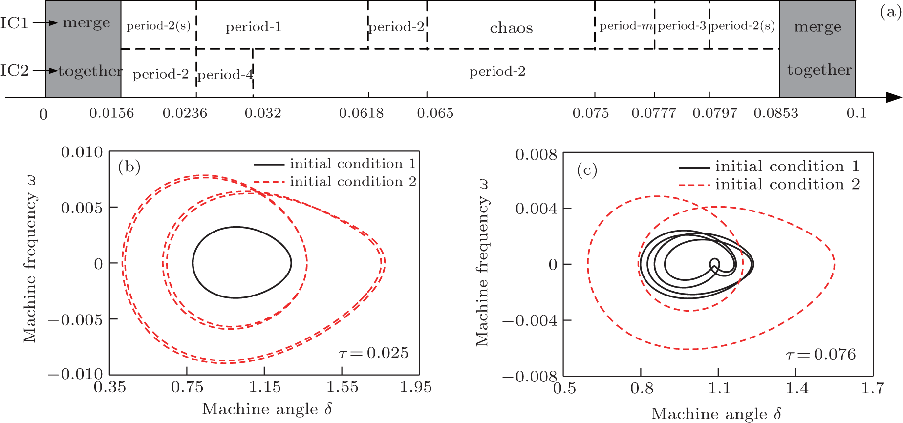 | Fig. 12. (a) Parameter domains of coexistence with τ varying (“ S” is small and “ m” is multiple). Coexisting motions of different periodic orbits, (b) τ = 0.025 and (c) τ = 0.076. |
From the above bifurcation diagrams and phase portraits, the different coexisting phenomena are presented with the mechanical power, damping factor, exciter gain, and time delay varying. One is the coexistence of two different periodic orbits, and the other is the coexistence of chaotic attractors and periodic orbits. When the system parameters are given as D= 2, KA= 150, and τ = 0.068, the coexisting domains with Pm ∈ [1.2, 1.356] are presented in the time-delayed power system, including the coexistance of chaos and period-2, chaos and period-4. With the damping factors D varying in the range of [0, 20] for Pm = 1.3, KA= 150, and τ = 0.068, the behaviors in the power system are shown the coexist of period-2 and chaos, period-2 and period-m. Similarly, when the exciter gain changes from 130 to 135 with Pm = 1.3, D= 2, and τ = 0.068, the only three types of coexisting phenomena are observed with period-1 and period-2, chaos and period-2, and two period-2 attractors with different structures. Finally, with the time delay τ increasing from 0 to 0.1, the same coexistance is also obtained in the power system but with diverse patterns.
The analysis of bifurcation behavior calculated for parameters Pm, D, KA, and τ allows us to reveal the following main properties in the power system. The discontinuous bifurcations are found in the time-delayed power system which indicates that the system has a jump of eigenvalues. The time-delayed power system is a multistable system which can exhibit abundant coexisting motions for a fixed set of parameters with different initial conditions. That is why the chaotic oscillation occurs in power systems and makes the system lose stability, even though in the normal operating parameter range the coexisting motions will not always exist in the power system and will disappear at certain parameters due to the crises eventually.
The nonlinear dynamic characteristics of a fourth-order time-delayed power system with the coexisting phenomenon are investigated in this paper. The bifurcation diagrams and phase portraits for different system parameters are displayed with different initial conditions to prove the existence of coexisting phenomenon in power systems. From the results, this coexistance of motions can only appear in some parameter’ s regions and then vanish at certain parameters. In particular, a “ jump” phenomenon is obtained to make the bifurcation diagrams break into pieces due to its discontinuous characteristics. In real power systems, the coexistence of different undesirable behaviors will stress the system component resulting in malfunctioning or crisis. The exact coexisting parameter intervals and regions given in this paper are useful to develop the practical design rule to avoid a certain type of mechanical oscillation, which will provide a good foundation for the future study of nonlinear time-delay power systems.
| 1 |
|
| 2 |
|
| 3 |
|
| 4 |
|
| 5 |
|
| 6 |
|
| 7 |
|
| 8 |
|
| 9 |
|
| 10 |
|
| 11 |
|
| 12 |
|
| 13 |
|
| 14 |
|
| 15 |
|
| 16 |
|
| 17 |
|
| 18 |
|
| 19 |
|
| 20 |
|
| 21 |
|
| 22 |
|
| 23 |
|
| 24 |
|
| 25 |
|
| 26 |
|
| 27 |
|
| 28 |
|
| 29 |
|
| 30 |
|
| 31 |
|
| 32 |
|
| 33 |
|
| 34 |
|
| 35 |
|