Approximate analytical solution of the Dirac equation with q-deformed hyperbolic Pöschl–Teller potential and trigonometric Scarf II non-central potential
[Kurniawan Ade†  , Suparmi A., Cari C.]
, Suparmi A., Cari C.]
|
|


†Corresponding author. E-mail: adekoerniawanzz92@gmail.com
An approximate solution of the Dirac equation for a spin-1/2 particle under the influence of q-deformed hyperbolic Pöschl–Teller potential combined with trigonometric Scarf II non-central potential is studied analytically. It is assumed that the scalar potential equals the vector potential in order to obtain analytical solutions. Both radial and angular parts of the Dirac equation are solved using the Nikiforov–Uvarov method. A relativistic energy spectrum and the relation between quantum numbers can be obtained using this method. Several quantum wave functions corresponding to several states are also presented in terms of the Jacobi Polynomials.
In quantum mechanics, it is well known that the Schrö dinger equation plays important roles for describing the behaviors of a particle at the microscopic scale. However, when the relativistic effect becomes important, the Schrö dinger equation should be replaced with relativistic wave equations, i.e., the Klein– Gordon equation for spin-0 particles and the Dirac equation for spin-1/2 particles, since the Schrö dinger equation is postulated for particles under a non-relativisic condition.[1] In particular, the Dirac equation has been applied to solve many problems in nuclear and high-energy physics. In solving the Dirac equation, some authors often assumed that the scalar potential is equal to the vector potential. Fishbane et al. have shown that the confining potential in the Dirac equation involving the interaction of fermions does not lead to Klein paradoxes if the strength of the vector potential is appropriately limited as compared to the scalar potential.[2] In the phenomenology of quarkonium, an equal mixture of vector potential and scalar confining potential leads to the best fit for the spin– orbit splittings of the spectrum.[3]
Recently, a large number of theoretical works were devoted to investigating analytical solutions of the Dirac equation with various potentials, including the Yukawa potential, [4, 5] the Woods– Saxon potential, [6– 8] the Hartmann potential, [9, 10] the Rosen– Morse type potential, [11] the Scarf-type potential, the Kratzer potential, [12] and various modifications of the spherical harmonic oscillator potential.[13– 19] The methods used in their studies included the standard method, [20] supersymmetry quantum mechanics, [13, 20] the path integral method, [21, 22] the Nikiforov– Uvarov method, [23– 25] and others.
The aim of this paper is to present the relativistic energy spectrum and spinor wavefunction of a spin-1/2 particle under bound state condition, by solving the Dirac equation with the q-deformed modified Pö schl– Teller potential and trigonometric Scarf II non-central potential using the Nikiforov– Uvarov (NU) method. Quantum deformation has a wide range of applications, including applications for nuclei, [26, 27] quantum-statistical theory, string/brane theory, and conformal field theory.[28, 29] It is assumed the role of the centrifugal term in the radial part of the Dirac equation, i.e., l ≠ 0. So, instead of solving the Dirac equation exactly, the hyperbolic approximation scheme[30] is used in order to obtain the radial solutions. It is also assumed in this paper that the scalar potential is equal to the vector potential. The basic strategy to obtain the solutions is reducing the Dirac equation to the hypergeometric-type equation with suitable changes of variables. Then the energy eigenvalue and the corresponding wavefunction can be derived using the Nikiforov– Uvarov method.
This paper is organized as follows. The Nikiforov– Uvarov method will be briefly reviewed in Section 2. In Section 3, we review the q-deformed hyperbolic function, give a brief introduction to the Dirac equation with equal scalar and vector potentials, and apply the separation of variables in spherical coordinates. In Section 4, we solve the radial and angular parts of the Dirac equation with the q-deformed modified Pö schl– Teller potential combined with trigonometric Scarf II non-central potential and obtain the relativistic energy spectrum and normalized spinor wavefunction via the Nikiforov– Uvarov method. In Section 5, we present graphically some normalized spinor wavefunctions of the Dirac equation, present several relativistic energy spectra, and discuss some consequences of the results obtained. Finally, the conclusions obtained are given in Section 6.
The one-dimensional Dirac equation of any shape invariant potential can be reduced into a hypergeometric or confluent hypergeometric type differential equation by suitable changes of variables. Nikiforov and Uvarov[31] introduced their method starting from the hypergeometric differential equation which has the form
where σ (s) and 


Substituting Eq. (2) into Eq. (1), one obtains a new equation of hypergeometric type

Here ϕ (s) is defined as the logarithmic derivative

And y(s) is a hypergeometric-type function, whose polynomial solutions are given by the Rodrigues relation

where Bn is the normalization constant, and ρ (s) is a weight function, which must satisfy

Function π (s) in Eq. (4) is defined as
 |
and parameter λ in Eq. (3) is defined as
 |
The k in Eq. (7a) can be found under the condition that the expression under the square root sign is the square of a polynomial. This is possible only if its discriminant is zero. The eigenvalues corresponding to the eigenfunctions defined in Eq. (5) are

where

The relativistic energy spectrum of the Dirac equation in hypergeometric form can be formulated by equating this eigenvalue equation (Eq. (8)) with Eq. (7b). The extra condition for Eq. (9) is that its derivative must be negative, i.e., τ ′ < 0. Thus, the quantum wavefunction can be obtained using Eq. (2) with Eq. (5) and the solution of ϕ (s) in Eq. (4).
The Dirac equation with scalar potential S(r) and vector potential V(r) (c = ħ = 1) is

where

in which σ is the vector Pauli spin matrix, and I is the identity matrix. In the Pauli– Dirac representation, let

we have
 |
 |
When the scalar potential is equal to the vector potential, equation (13) becomes
 |
 |
Substituting Eq. (14b) into Eq. (14a) yields

In spherical coordinates, the q-deformed modified Pö schl– Teller potential combined with the trigonometric Scarf II non-central potential is defined as
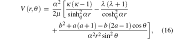
where b2 + a(a − 1), b(2a − 1), κ , and λ are positive real numbers. Putting Eq. (16) into Eq. (15) and simplifying the equation, we have


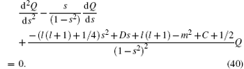
with
Let

separating the variables in Eq. (17), we obtain
 |
 |
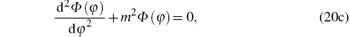 |
where ε 2 = − (E2 − μ 2c4). Equation (20c) is well known with its solution

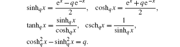
The q-deformed hyperbolic functions, used as one of the parameters in the modified Pö schl– Teller central potential, are defined by[24]
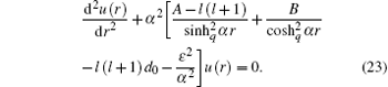
The radial part of the Dirac equation with the q-deformed modified Pö schl– Teller central potential contains the centrifugal term l(l + 1)/r2 since we assume l ≠ 0. However, the Pö schl– Teller potential is a kind of potential which cannot be solved exactly when the centrifugal term is taken into account unless l = 0 is assumed. The conventional approximation used in this paper is

Substituting Eq. (22) into Eq. (20a) and simplifying the equation, we have
To transform Eq. (23) to a hypergeometric-type equation, a new variable is introduced, i.e., 

The associated polynomials can be obtained by comparing Eqs. (24) and (1), we obtain
 |
 |
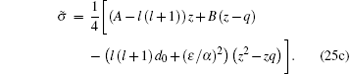 |
By substituting Eq. (25) into Eq. (7a) and simplifying the equation, we obtain
with
 |
 |
The quadratic expression under the square root of Eq. (26) must be the completed square of a first degree polynomial, provided that the discriminant of this quadratic expression equals zero
The k in Eq. (26) is obtained by expanding and solving quadratic equation (28), where two solutions of Eq. (28) for k can be written as follows:

Substituting the k in Eq. (29) into Eq. (26), we obtain four solutions to the first-order as follows:

for
for

Since the appropriate solution of π (z) requires that the derivative of τ (Eq. (9)) is negative, we choose π 2(z) with a negative sign, i.e.,

with

Substituting Eq. (30) into Eqs. (7b) and (9) together with Eq. (25a), then putting Eq. (9) into Eq. (8), we obtain two equations for λ ,
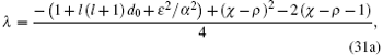 |
 |
Since both λ and λ n in Eq. (31) are equivalent, we can equate Eqs. (31a) and (31b). Thus after mathematical manipulation, we obtain the relativistic energy spectrum

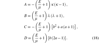
where we have replaced ε 2 with – (E2 – μ 2). By substituting Eqs. (18) and (27) into Eq. (32), we obtain the complete form of the relativistic energy spectrum as follows:
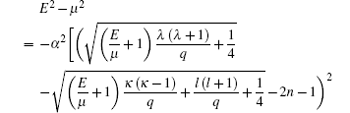

Equation (33) is the bound state relativistic energy spectrum for a spin-1/2 particle under the influence of the q-deformed modified Pö schl– Teller potential, which is mathematically equivalent to that obtained by Zhang et al.[10] using supersymmetry quantum mechanics in the case of l = 0 and q = 1. The energy can be obtained numerically or graphically.
To obtain the radial wavefunctions of the Dirac equation, first we determine the weight function using Eq. (6) as follows:

Substituting Eq. (34) above into Eq. (5), we have

where Bn is the normalization constant. Using Eq. (4), we have

Finally, we obtain the radial part of the wavefunction, u(r) = ϕ (r)yn(r), with Eq. (35) defined in terms of Jacobi polynomials 
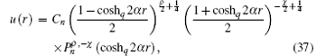
where Cn is the radial normalization constant. The radial wavefunction presented in Eq. (37) is a result based on the conventional approximation used for the centrifugal term, that is, by replacing centrifugal term l(l + 1)/r2 with Eq. (22). In the case of an exact solution, one can choose the value of l to be zero, and equation (37) will transform into the exact form. This form is mathematically equivalent as obtained by Zhang et al.[10] using supersymmetry quantum mechanics.
The angular part of the Dirac equation cannot be defined in terms of spherical harmonics in this paper since the particle is under the influence of a non-central potential, i.e., the trigonometric Scarf II potential, which is defined in Eq. (16). Fortunately, the angular part of the Dirac equation can be solved exactly using the Nikiforov– Uvarov method. To transform Eq. (20b) into the hypergeometric form, first we simplify the equation for θ by substituting

into Eq. (20b), which yields
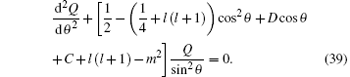
To transform Eq. (39) into a hypergeometric-type equation, we define a transformation variable s = cosθ . Substituting it into Eq. (39), we have
As we did before, the associated polynomials can be obtained by comparing Eqs. (40) and (1)
 |
 |
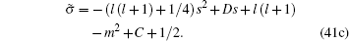 |
By substituting Eq. (41) into Eq. (7a) and simplifying the equation, we obtain

The quadratic expression under the square root of Eq. (42) must be the completed square of a first degree polynomial, provided that the discriminant of this quadratic expression equals zero

The k in Eq. (42) is obtained by expanding and solving quadratic equation (43). Two solutions of Eq. (43) for k can be written as follows:

where
 |
 |
Substituting Eq. (44) into Eq. (42), we obtain four solutions to the first-order as follows:
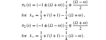
Since the appropriate solution of π (s) requires that the derivative of τ (Eq. (9)) is negative, we choose π 1(s) with a negative sign, i.e.,


Substituting Eq. (46) into Eqs. (7b) and (9) together with Eq. (41a), then putting Eq. (9) into Eq. (8), we have two equations for λ ,
 |
 |
By equating Eqs. (47a) and (47b), the relation between quantum numbers corresponding to the angular part of the Dirac equation can be obtained as follows:

where 
The weight function corresponding to the solution of the angular part of the Dirac equation is

Substituting Eqs. (41b) and (49) into Eq. (5) yields

where Bñ is the normalization constant. Using Eq. (4), we have

Now, we obtain the angular part of the wavefunction Q(θ ) = ϕ (θ )yñ (θ , ). With Eq. (51) defined in terms of Jacobi polynomials 
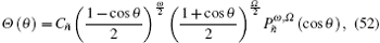
where Cñ is the angular normalization constant.
Finally, we have the complete spinor wavefunction of the Dirac equation for a particle under the influence of the q-deformed modified Pö schl– Teller potential and trigonometric Scarf II non-central potential, i.e.,
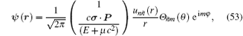
where u(r) and Θ (θ ) have been given in Eqs. (37) and (52).
In this section, we discuss several results obtained in the previous section. By varying parameter α , ρ and χ defined in Eq. (27) and defining coshq2α r = p, some of the radial wavefunctions are listed in Table 1.
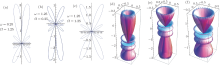
 | Fig. 1. (a)– (c) Polar diagrams and (d)– (f) three-dimensional representations of the angular wave function for a state n = 4 with varing ω and Ω . In panels (a) and (d), ∣ Θ (θ )∣ 2 = 1.97022(1.61865 + 16.834(− 1 + cosθ ) + 42.085(− 1 + cosθ )2 + 36.6895(− 1 + cosθ )3 + 10.2515(− 1 + cosθ )4)2(1 − cosθ )0.25(1 + cosθ )1.25; in panels (b) and (e), ∣ Θ (θ )∣ 2 = 1.97022(6.79834 + 39.2793(− 1 + cosθ ) + 67.9834(− 1 + cosθ )2 + 45.3223(− 1 + cosθ )3 + 10.2515(− 1 + cosθ )4)2(1 − cosθ )1.25(1 + cosθ )0.25; in panels (c) and (f), ∣ Θ (θ )∣ 2 = 1.33582(6.79834 + 45.3223(− 1 + cosθ ) + 88.9014(− 1 + cosθ )2 + 66.2402(− 1 + cosθ )3 + 16.5601(− 1 + cosθ )4)2(1 – cosθ )1.25(1 + cosθ )1.25. |
| Table 1. Radial wave functions corresponding to several states of a particle under the influence of the q-deformed hyperbolic Pö schl– Teller potential and trigonometric Scarf II potential. |
| Table 2. Energy eigenvalues corresponding to several states of a particle under the influence of q-deformed Pö schl– Teller potential and trigonometric Scarf II potential. |
The sign of deformed parameter q in the Pö schl– Teller potential does not affect the radial part of the spinor wavefunction due to the square term of q contained in coshq2α r,

Equations (33) and (48) constitute a complete relativistic energy spectrum, which can be obtained numerically. Several examples of energy eigenvalue are listed in Table 2 with parameters λ = 1, κ = 1.5, a = 0.75, b = 0.25, and μ = 10 fm− 1, the positive value is taken due to the spin symmetric limit.
For the angular solution of the spinor wavefunction, we compare three spinor wavefunctions with the same quantum number ñ = 4 but varying ω and Ω in Fig. 1. The plot is displayed in two and three dimensions together with the wavefunction.
By inspecting Fig. 1, the variation of ω and Ω for the angular part of the spinor wavefunction influences the shape of the orbital probability distribution in space. From Eq. (45), ω and Ω are related with the strength of the Scarf II trigonometric potential. The asymmetry of ω and Ω in the angular part of the spinor wavefunction results in the asymmetry of the probability distribution in space. The asymmetry is clearly displayed in the two-dimensional plot.
In this paper, we study the Dirac equation for a spin-1/2 particle in the q-deformed hyperbolic Pö schl– Teller potential combined with the trigonometric Scarf II non-central potential under the condition that the scalar potential equals to the vector potential. The radial part of the spinor wavefunction is obtained approximately from Eqs. (37) and (52). It is shown that the sign of q does not affect the wavefunction. However, the sign of parameter q affects the relativistic energy spectrum. The angular part of the spinor wavefunction can be obtained exactly and an important discussion corresponding to the asymmetry of the probability distribution has been presented in Section 5.
| 1 |
|
| 2 |
|
| 3 |
|
| 4 |
|
| 5 |
|
| 6 |
|
| 7 |
|
| 8 |
|
| 9 |
|
| 10 |
|
| 11 |
|
| 12 |
|
| 13 |
|
| 14 |
|
| 15 |
|
| 16 |
|
| 17 |
|
| 18 |
|
| 19 |
|
| 20 |
|
| 21 |
|
| 22 |
|
| 23 |
|
| 24 |
|
| 25 |
|
| 26 |
|
| 27 |
|
| 28 |
|
| 29 |
|
| 30 |
|
| 31 |
|