Inverse problem of pulsed eddy current field of ferromagnetic plates*
[Chen Xing-Le†  , Lei Yin-Zhao]
, Lei Yin-Zhao]
|
|


†Corresponding author. E-mail: chenxingle@yeah.net
*Project supported by the National Defense Basic Technology Research Program of China (Grant No. Z132013T001).
To determine the wall thickness, conductivity and permeability of a ferromagnetic plate, an inverse problem is established with measured values and calculated values of time-domain induced voltage in pulsed eddy current testing on the plate. From time-domain analytical expressions of the partial derivatives of induced voltage with respect to parameters, it is deduced that the partial derivatives are approximately linearly dependent. Then the constraints of these parameters are obtained by solving a partial linear differential equation. It is indicated that only the product of conductivity and wall thickness, and the product of relative permeability and wall thickness can be determined accurately through the inverse problem with time-domain induced voltage. In the practical testing, supposing the conductivity of the ferromagnetic plate under test is a fixed value, and then the relative variation of wall thickness between two testing points can be calculated via the ratio of the corresponding inversion results of the product of conductivity and wall thickness. Finally, this method for wall thickness measurement is verified by the experiment results of a carbon steel plate.
In industry, corrosive media with high temperature and high pressure usually stored and transported by ferromagnetic containers and pipes, and wall-thinning corrosion of ferromagnetic components is a widespread and unavoidable damage. Therefore, a regular in-service nondestructive testing on the remaining wall thickness is indispensable to ensure safe operation. Pulsed eddy current testing (PECT) is an effective electromagnetic nondestructive method for inspecting coated ferromagnetic containers and pipes.[1– 4] A pulsed magnetic field is excited by a pulsed current, instead of a sinusoidal excitation current; and then, by detecting this transient electromagnetic field, the wall-thinning corrosion of the component could be detected. The study results in Ref. [5] point out that the time-domain voltage induced by a pulsed excitation current is greatly more sensitive to the wall thickness of ferromagnetic components, compared with the frequency-domain voltage induced by a sinusoidal current.
The determination of electromagnetic parameters and wall thickness of the component under test is the key for signal processing in PECT. Much research in recent years has focused on extracting features directly from the signal. Reference [2] extracts two time constants from the logarithmic scaled induced voltage signal and try to determine both material properties and absolute wall thickness of a steel plate simultaneously. The decay rate estimated from the semi-logarithmic scaled signal over a certain time is used to evaluate the wall thickness of insulated carbon steel pipes.[3] In addition, the wall-thinning corrosion of insulated ferromagnetic pipes may be assessed by the time-to-peak of the differential signal.[4] These methods have the advantages of simple and fast signal processing; unfortunately, it is hard to get the expressions of these signal features, hence the testing results are easily influenced by a change in parameters such as the conductivity and permeability of the ferromagnetic component under test, and the lift-off of the probe. Based on time-domain analytical solutions to PECT models, this paper tries to determine the parameters of ferromagnetic plates by establishing an inverse problem with measured values and calculated values of the time-domain signal.
For axisymmetric eddy current problems, a classical method is proposed in Refs. [6] and [7] to achieve the closed-form expressions of the magnetic vector potential by the separation of variables. Rather than an integral form as in Ref. [6], modified expressions for conducting plates in the form of a series are obtained by the TREE method (truncated region eigenfunction expansion).[8, 9] However, the method in Ref. [6] is no longer appropriate to solve non-axisymmetric eddy current field problems such as cylindrical and tubular conductors. Fortunately, second-order vector potential (SOVP) has been proved to be an effective tool to solve these models; analytical solutions to the impedance of the probe coil positioned outside a conducting cylinder are obtained by the SOVP formulation.[10, 11]
For the linear transient eddy current electromagnetic field, the well-posedness of the initial-boundary value problem is investigated.[12, 13] Through the Laplace inverse transformation, time-domain solutions to the pulsed eddy current field can be calculated from their frequency-domain solutions.[14– 18] For example, time-domain analytical solutions to the pulsed magnetic field for planar slabs and enclosures are obtained via the Laplace inverse transformation, which is carried out through the residue theorem.[14] Furthermore, using the Heaviside expansion theorem, a method for solving the time-domain pulsed eddy current field of a conducting plate was proposed in Refs. [15], [16], and [18]. Moreover, through the SOVP formalism and Laplace inverse transformation, the non-axisymmetric pulsed eddy current field induced by a probe coil positioned perpendicularly outside a conducting ferromagnetic pipe is solved analytically.[19]
The analytical solutions mentioned above have the advantages of high speed, high precision, and derivable for calculating. Based on the time-domain analytical solutions to the PECT model of ferromagnetic plates, this paper tries to determine the wall thickness, conductivity and permeability of the ferromagnetic plate by establishing a least squares problem between the measured values and calculated values of time-domain induced voltage. This paper is organized as follows. In Section 2, the time-domain solutions to the PECT model of a ferromagnetic plate are introduced. Next, the least squares problem is established, then, the dependence relation of partial derivatives with respect to parameters is discussed and the constraints of parameters are given in Section 3. Furthermore, with and without constraints, the sensitivity to the wall thickness of the time-domain induced voltage are compared in Section 4. Finally, the method proposed in this paper for measuring the relative wall thickness is verified by experimental results in Section 5, and the conclusions are given in Section 6.
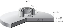
The PECT model of a conducting, ferromagnetic plate is studied in this paper as shown in Fig. 1. Respectively, the wall thickness, conductivity, and permeability of the ferromagnetic plate under test are denoted as d, σ , and μ , where μ = μ 0μ r (μ 0 is the permeability of the vacuum, and μ r is the relative permeability of the plate). A cylindrical pick-up coil (subscript p) and drive coil (subscript d) of height h are positioned perpendicularly above the plate. lo is the lift-off between the probe and the upper surface of the plate. The geometric parameters of the air-cored probe coil are listed in Table 1. A cylindrical coordinate system Oρ φ z is established, and its z-axis is coincident with the central axis of the probe. Following the TREE method in Ref. [8], a magnetic insulation boundary is imposed on the surface ρ = b to truncate the solution region of the PECT model as in Fig. 1, where b is set to be 5 to 10 times larger than the radius of the probe coil to have a sufficient calculation accuracy.
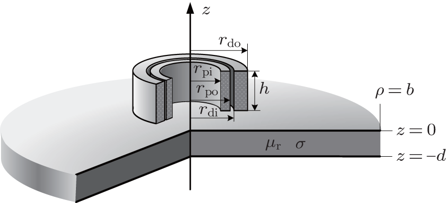 | Fig. 1. The PECT model of two air-cored cylindrical coils positioned perpendicularly above a conducting ferromagnetic plate. |
| Table 1. Geometric parameters of the probe coils. |
In the PECT on a ferromagnetic plate, a pulsed eddy current field is excited by a pulsed current in the drive coil, then, the wall-thinning corrosion of the plate under test can be detected through the induced voltage across the pick-up coil.
With respect to the axisymmetric eddy current field as in Fig. 1, the magnetic vector potential A only has a circumferential component Aφ , i.e., A = Aφ eφ . Here, I(s) is the Laplace transform of excitation current i(t) excited in the drive coil. Ignoring the displacement current, under zero initial conditions, Aφ in the frequency-domain satisfies[7]

where k2 = – μ σ s, in the conducting regions, and k2 = 0, in the non-conducting regions. Following the previous work, the complex frequency-domain expansions for the truncated eddy current field shown in Fig. 1 have been obtained.[15, 18] Then, through the Laplace inverse transformation, the time-domain induced voltage of the pick-up coil can be solved as[5, 18]

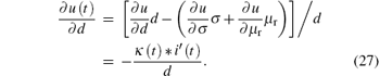
where i′ (t) is the time derivative of excitation current i(t), and “ * ” denotes the convolution algorithm, 
where ξ k denotes the k-th positive root of the transcendental equation

where 

Cd(λ i) and Cp(λ i) given in Refs. [15] and [18] are called coil coefficients of the drive and pick-up coils, respectively. They have the same expression, which only depends on geometric parameters and the lift-off of the probe coils, and is independent of the parameters of the plate under test.
The minor hysteresis curves of ferromagnetic materials under pulsed excitation current are measured in Ref. [20], and measurement results indicate that magnetization curves of ferromagnetic materials under a periodic pulsed excitation current are a minor loop with a leaf shape. Here, the minor loop of the ferromagnetic plate under pulsed magnetic field has been linearized approximately, and the relative permeability of the ferromagnetic plate is simplified to be an unknown parameter μ r.[21] Generally speaking, the relative permeability will be influenced by factors such as microstructural properties, pulsed excitation magnetic field, and pre magnetization. Hence, the relative permeability μ r of the ferromagnetic plate under test is a variable parameter and hard to be measured, here μ r is set to be an unknown parameter which will be determined by the inverse problem in this paper.
In the PECT model shown in Fig. 1, wall thickness d, conductivity σ , and relative permeability μ r of the ferromagnetic plate under test are unknown parameters to be determined, hence set an unknown parameter vector x = (d, σ , μ r)T. The purpose of PECT on ferromagnetic plates is to determine the unknown parameter vector x by the testing signal, and then the wall-thinning corrosion of the plate can be evaluated by the inverse results of the wall thickness. We estimate the unknown parameters by a least squares method from the time-domain induced voltage with values (t1, u1) (t2, u2), … , (tm, um) collected by a data acquisition card. The least squares problem requires that
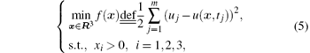
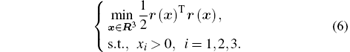
where u(x, t) is the theoretical value of induced voltage calculated by Eq. (2). Defining residues rj (x) = uj − u(x, tj) j = 1, 2, … , m, and a residue vector r(x) = (r1(x), r2(x), … , rm(x))T, the least squares problem can be rewritten as
The gradient of the objective function f(x) is

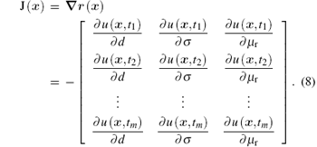
where J(x) is the Jacobian matrix of the residue vector r(x)
The necessary condition for a local minimum point x* of the sum of residual squares f(x) is

and it leads to a non-linear equation system which must be solved by an iterative method, e.g., by the Gauss– Newton method. It is necessary to study the uniqueness and stability of the solution of inverse problem (5) before we choose a numerical algorithm. Equation (9) indicates that the Jacobian matrix J(x) is the key for studying the properties of the local minimum point x* .
Equation (8) indicates that solving the Jacobian matrix J(x) is equivalent to solving the partial derivatives of induced voltage with respect to the parameters in x, i.e.,

In Eq. (2), the voltage induced by the incident field and reflection field is independent of the parameters in x, hence
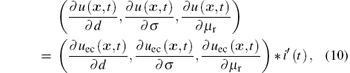
it indicates that solving the partial derivatives of induced voltage u(x, t) with respect to the parameters can be transformed into solving the partial derivatives of the voltage induced by eddy current field uec(x, t). From Eq. (3), the partial derivative of the induced voltage uec(x, t) with respect to the conductivity σ can be derived directly as
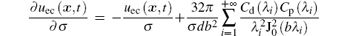
For solving the partial derivative with respect to wall thickness, firstly, using the implicit function theorem the partial derivatives of roots ξ k with respect to the wall thickness d should be solved as

and then, from Eq. (3), the partial derivative of the induced voltage uec(x, t) with respect to the wall thickness d can be derived as

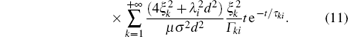
where
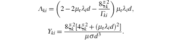
Similarly, the partial derivatives of roots ξ k with respect to the relative permeability μ r can be solved as

and then the partial derivative of the induced voltage uec(x, t) with respect to the relative permeability μ r can be derived as
where

Substituting the partial derivatives calculated by Eqs. (11), (13), and (15) into Eq. (10), the Jacobian matrix J(x) of the inverse problem (5) can be obtained. The residue function r(x) can be approximated in the neighborhood of the local minimum point x* by the linear part of its Taylor expansion with respect to x, so the linearization of r(x) can be given by

thus the non-linear least squares problem (5) is translated into a linear east squares problem. From the optimality condition of the linear least squares problem, if the columns of the coefficient matrix J(x* ) in Eq. (16) are linearly dependent, the local minimum point of this inverse problem will not be unique. Therefore, the dependence relation of the partial derivatives is important for solving the inverse problem. Defining a function κ (t) as

Substituting Eqs. (11), (13), and (15) into κ (t), many common factors of the partial derivatives can be removed, and κ (t) has a very simple expression as
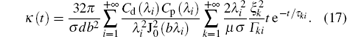
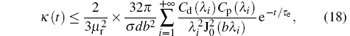
The study results in Ref. [5] point out that the effects of all ξ k and τ ki can be estimated by the first positive root of Eq. (4) as ξ 1 ≈ π /2, and the diffusion time constant of the pulsed eddy current in ferromagnetic plates as τ e = μ σ d2/π 2. Due to the restriction of acquisition precision, only the voltage signal within 3τ e should be collected in the PECT, so here t ≤ 3τ e, and then the upper limit of Eq. (17) can be calculated approximately as
where the coefficient

only depends on the geometric parameters and lift-off of the probe coils. The same as the induced voltage uec(x, t) and its partial derivatives

equation (18) has the coefficient

which is calculated of the 100 order of magnitude. Therefore, the upper limit of κ (t) is close to 0 as the relative permeability of ferromagnetic materials commonly satisfies μ r≫ 1, hence κ (t) ≈ 0 holds.
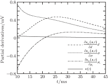
A set of parameters of a steel plate under test is supposed as d = 8 mm, σ = 6 MS/m, and μ r = 200. In Table 1, the geometric parameters of the air-cored probe coils are listed, and the lift-off of the probe lo is 10 mm. Respectively, the partial derivatives calculated by Eqs. (11), (13), and (15) are plotted in Fig. 2. The solid line in Fig. 2 denotes κ (t) calculated by Eq. (17). Comparing these curves, it can be seen that κ (t) ≈ 0 holds, i.e.,

 | Fig. 2. Partial derivatives of the voltage induced by eddy current field with respect to parameters. |
As shown in Eq. (19), the results obtained above indicate that the partial derivatives of the induced voltage signal with respect to the parameters are approximately linearly dependent, in the PECT on ferromagnetic plates. It leads to a very large condition number for the Jacobian matrix J(x), then the solution of inverse problem (5) will have a large relative error, namely, a large error of the inversion results of parameters would be caused by a small error in the testing signal. In order to demonstrate this conclusion, substituting Eq. (19) into Eq. (10), and supposing

Solutions to this homogeneous partial linear differential equation are equivalent to solutions of the so-called characteristic system[22]
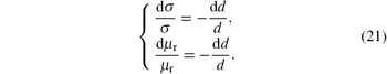
This system can be solved by first integrals as

where C1 and C2 are arbitrary constants. Every first integral (22) of the system (21) is a solution to the homogeneous linear partial differential equation (20), if these two integrals are independent, then the general solution of Eq. (20) is

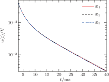
This indicates that induced voltage can be expressed as a function up of two arguments σ d and μ rd. Let xp = (σ d, μ rd)T, then the induced voltage u(x, t) can be expressed as up(xp, t). In the calculation model described in Section 3.3, the parameters of the ferromagnetic plate under test are supposed as x1 = (8 mm, 6 MS/m, 200)T, x2 = (6 mm, 8 MS/m, 267)T, and x3 = (10 mm, 4.8 MS/m, 160)T respectively. Obviously, these sets of parameters correspond to the same xp = (4.8 × 10⁴ S, 1.6 m)T. An exponential decaying pulsed current with an amplitude of 4.0 A and a fall time of 0.62 ms is excited in the drive coil. Theoretical curves of the induced voltage calculated by Eq. (2) with different sets of parameters x1, x2, and x3 are plotted in Fig. 3. These theoretical curves of the induced voltage are barely distinguishable, as the parameters of the ferromagnetic plate under test satisfy the constraints (22). Conversely, in the PECT on ferromagnetic plates, only the product of conductivity and wall thickness σ d, and the product of relative permeability and wall thickness μ rd, i.e., xp, can be determined by establishing the inverse problem (5) with the measured values and calculated values of time-domain induced voltage signal.
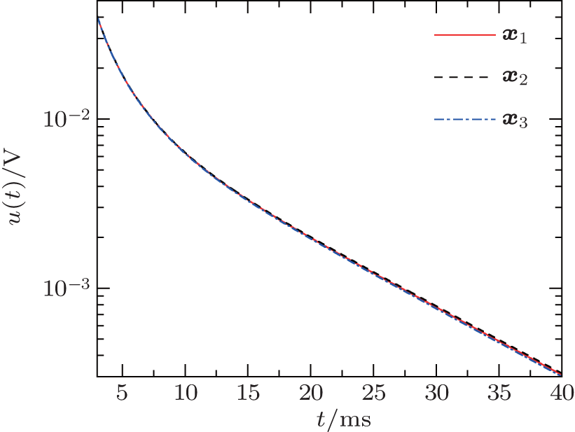 | Fig. 3. Theoretical calculation curves of the induced voltage with different sets of parameters (x1 = (8 mm, 6 MS/m, 200)T, x2 = (6 mm, 8 MS/m, 267)T, and x3 = (10 mm, 4.8 MS/m, 160)T). |
From Fig. 3, it can be observed visually that the time-domain induced voltage is significantly insensitive to wall thickness d when the parameters in x satisfy the constraints (22). Next, with and without the constraints (22), the sensitivity of the time-domain induced voltage u(t) to wall thickness d will be compared. In order to estimate the sensitivity quantitatively, we formulate the partial derivative ∂ u(t)/∂ d and normalized derivative ζ d(t) of induced voltage with respect to wall thickness, where the normalized derivative is defined as

which denotes the relative variation of the induced voltage caused by a relative change in wall thickness. Without the constraints of parameters, the partial derivative can be given by

where ∂ uec(x, t/∂ d is calculated by Eq. (13). On the other hand, with the constraints of parameters as shown in Eq. (22), we have σ = C1/d and μ r = C2/d, substituting them into u(x, t)

supposing only the variable d is changing, other variables are considered as constants, then the partial derivative with respect to wall thickness d can be deduced as
Substituting Eq. (27) into Eq. (24), we have

Similarly, solving the partial derivatives with respect to conductivity σ and relative permeability μ r under the constraints (22), and then substituting them into Eq. (24), we have

From Eqs. (28) and (29), it is obvious that when the parameters in x satisfy the constraints (22), the variation and relative variation of the induced voltage caused by a relative change in parameters can be calculated by κ (t). Hence, the sensitivities of induced voltage to the parameters can be estimated by κ (t). From Eqs. (17) and (3), the difference between κ (t) and uec(t) is a coefficient 


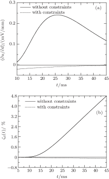
In the calculation model described in Section 3.4, the parameters of the plate under test are supposed as x = (8 mm, 6 MS/m, 200)T. Respectively, with and without the constraints (22), the variation curves of the time-domain induced voltage caused by a 1 mm change in wall thickness are calculated by Eqs. (25) and (27), and are plotted in Fig. 4(a); the normalized variation curves caused by a 1% relative change in wall thickness are calculated by substituting Eqs. (25) and (27) into Eq. (24), and are plotted in Fig. 4(b). From Fig. 4, it is evident that when the parameters in x satisfy the constraints (22), the sensitivity of the induced voltage to wall thickness will be significantly reduced. Furthermore, the variation and normalized variation of the testing signal caused by a change in wall thickness is so slight, and easily disturbed by noise. Here, even though using a data acquisition card with an accuracy of 0.05 mV, it is incapable of detecting a 1 mm change (equivalent to 12.5% relative change) in wall thickness by the time-domain induced voltage.
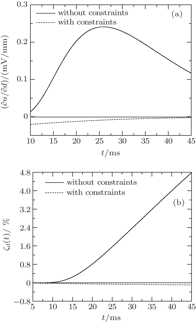 | Fig. 4. With and without the constraints, the variation curves of the time-domain induced voltage caused by a 1 mm change in wall thickness (a), and the normalized variation curves caused by a 1% relative change in wall thickness (b). |
In the practical PECT, an inevitable error between theoretical calculated values and experimental measured values of the time-domain induced voltage is usually caused by many factors, such as the resolution and accuracy of the data acquisition board, electromagnetic and circuit noise, and the model error caused by linearizing the minor magnetization curve of the ferromagnetic plate. If we inverse three parameters in x simultaneously, it is difficult to distinguish the wall thickness which satisfies the constraints (22); and a small error in the induced voltage signal will lead to a large relative error in inversion results. Therefore, only the arguments σ d and μ rd can be determined accurately through the time-domain induced voltage signal carrying an error.
Supposing the conductivity σ of the ferromagnetic plate is a known constant, and the wall thickness d and the relative permeability μ r are unknown parameters to be determined, now the sensitivity curves of the induced voltage to the wall thickness d are the solid lines as shown in Fig. 4. Obviously, the sensitivity of induced voltage to the parameters will be significantly improved when setting a parameter in x e.g., conductivity σ to be a known constant. In the PECT on ferromagnetic plates, supposing the conductivity σ of the ferromagnetic plate under test is a fixed value, and then, the relative variation of the wall thickness between two testing points can be obtained via the ratio of the corresponding inversion results of the product of conductivity and wall thickness.
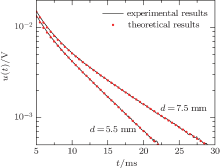
In the PECT experiments, a 1.0 m × 0.5 m × 7.5 mm carbon steel plate was tested, and half of the plate was milled to 5.5 mm in thickness. Then, comparison experiments could be carried out at two testing points with the same material and with wall thicknesses of 5.5 mm and 7.5 mm, respectively. The air-cored probe coils were positioned perpendicularly above the steel plate, with the lift-off lo of 20.0 mm between the probe coils and the upper surface of the plate. Geometric parameters of the cylindrical coils are shown in Table 1. Using an impedance analyzer, the drive coil’ s inductance and resistance in air were measured of 1.21 mH and 5.81 Ω , respectively. In the drive coil, a direct current with an amplitude of 4.0 A was shut off at the time point t = 0, and an exponential decaying pulsed current with an amplitude of 4.0 A and a fall time of 0.62 ms was excited. Then, the induced voltage across the pick-up coil was collected by a data acquisition card with a resolution of 16-bits. The measured results of induced voltage at two testing points with different wall thicknesses are plotted in Fig. 5.
 | Fig. 5. Experimental and theoretical calculation results of the time-domain induced voltage at two testing points with wall thicknesses of 5.5 mm and 7.5 mm respectively. |
The conclusions obtained in Section 4 point out that only two parameters in x can be determined via the time-domain induced voltage. Here, we set the product of conductivity and wall thickness σ d, and the product of relative permeability and wall thickness μ rd were unknown parameters to be determined by the inverse problem (5). Using the experimental results of the induced voltage in Fig. 5, the arguments σ d at two testing points with wall thicknesses of 5.5 mm and 7.5 mm were determined as 3.18 × 10⁴ S and 4.39 × 10⁴ S, respectively, and the corresponding μ rd were determined as 1.17 m and 1.27 m. Substituting the inversion results into Eq. (2), the theoretical curves of the induced voltage at two testing points were calculated and plotted in Fig. 5. The calculated results agree well with the measured results; it is verified that the inversion results are the solutions to the inverse problem (5). The ratio of the wall thickness between two testing points calculated via inversion results is 3.18 × 10⁴/4.39 × 104 = 72.4% ; actually, the ratio of the wall thickness between two testing points is 5.5/7.5 = 73.3% . This result presents a 0.9% error in the measurement, and indicates that it is feasible for the PECT method proposed in this paper to measure the relative variation of the wall thickness for ferromagnetic plates.
In the PECT on ferromagnetic plates, respectively, the partial derivatives of the time-domain induced voltage with respect to the wall thickness, conductivity, and relative permeability of the plate are solved analytically. From their expressions and theoretical calculation curves, it is indicated that the partial derivatives are approximately linearly dependent. On this basis, the constraints of the parameters are given by solving a homogeneous partial linear differential equation, and we point out that the induced voltage can be expressed as a function of two arguments. Next, the sensitivity of the induced voltage to wall thickness with and without the constraints is compared; theoretical analysis indicates that the relative variation of the induced voltage caused by a change in parameters is significantly slight when the parameters satisfy the constraints; through the inverse problem with the time-domain induced voltage, only the product of conductivity and wall thickness, and the product of relative permeability and wall thickness can be determined accurately in the practical PECT. Finally, experiment results verify the method that the relative variation of the wall thickness between two testing points can be calculated via the ratio of the corresponding inversion results of the product of conductivity and wall thickness. This method for wall thickness measurement is very useful for the PECT on the wall-thinning corrosion of ferromagnetic metallic pipes and containers.
| 1 |
|
| 2 |
|
| 3 |
|
| 4 |
|
| 5 |
|
| 6 |
|
| 7 |
|
| 8 |
|
| 9 |
|
| 10 |
|
| 11 |
|
| 12 |
|
| 13 |
|
| 14 |
|
| 15 |
|
| 16 |
|
| 17 |
|
| 18 |
|
| 19 |
|
| 20 |
|
| 21 |
|
| 22 |
|