
Controlling cooperativity of a metastable open system coupled weakly to a noisy environment*
[Teslenko Victor I.a)†  , Kapitanchuk Oleksiy L.
a)‡ , Yang Zhaob)§ ]
, Kapitanchuk Oleksiy L., Yang Zhao]
|
|


Corresponding author. E-mail: vtes@bitp.kiev.ua
Corresponding author. E-mail: alkapt@bitp.kiev.ua
Corresponding author. E-mail: yzhao@ntu.edu.sg
Project supported by the National Academy of Sciences of Ukraine (Grant No. 0110U007542) and the National Research Foundation of Singapore through the Competitive Research Programme (Grant No. NRF-CRP5-2009-04).
The notion of cooperativity comprises a specific characteristic of a multipartite system concerning its ability to demonstrate a sigmoidal-type response of varying sensitivities to input stimuli in transitions between states under controlled conditions. From a statistical physics viewpoint, in this work we attempt to describe the cooperativity by the stability of a metastable open system with respect to irreversibility. To treat the evolution of a system weakly coupled to the environment in a kinetic framework, we consider two fluctuating energy levels of different dimensionalities, initial population of one level, reversible transitions of population between the levels, and irreversible depopulation of another level. An average is made over level fluctuations and environment vibrations so that an inter-level transition rate can be obtained accounting for the influences of external control on level position and dimensionality. It is found that the cooperativity of the two-level system is bounded approximately between 0.736 and unity, with the lower bound indicating worsening system stability.
Collective dynamics, inherent in multipartite systems, is found in many fields such as physics, chemistry, biology, informatics, economics, medicine, and sociology. In molecular structures, for example, collectivity is featured by measures to characterize cooperative properties of systems in equilibrium.[1– 4] Such measures, usually named cooperativity indices or cooperativity degrees, are associated with the steepness of saturated system responses to experimentally controlled stimuli when fitting deviations of observed sigmoidal stimulus-response curves from a two-state Boltzmann distribution. Supporting examples are the Hill coefficient originally introduced to fit a ligand binding in multi-site proteins, [5] the elasticity coefficient fitting a response of relevant state variables to a change in control variables, [6] the strength of intermolecular interactions describing a functional promotion, or constraining of population of relevant states in respect with irrelevant ones, [7– 9] etc.
There may be two formal ways to treat equilibrium cooperative processes at the molecular level (cf. Ref. [10]). Firstly, the Boltzmann population distribution for a relevant state can be approximated by the normalized rational function of degree one, which corresponds to a few-state system with the cooperativity degree attributed to a control parameter involved in the distribution denominator via equilibrium constants and indexed as the maximum power of its integral series (greater than or equal to one, and less than the number of system states minus one). Within the second approach, the shape of the Boltzmann distribution cannot be approximated by that of a sigmoidal type, a case corresponding to a multistate system, in which the degree of cooperativity cannot be associated with some constant integer, but rather, with a variable that is fractional in value, and dependent on control parameters. The latter case includes a two-state system, for which a common consensus exists that the cooperativity degree would be one and only one regardless of the control parameters used for its evaluation.[11, 12] This implies that in equilibrium the two energy levels are statistically independent, and show no correlation or cooperativity beyond what is prescribed by the Boltzmann statistics.[13]
Cooperative systems, however, are not static in time and space. Instead, they temporally function in an equilibrium environment characterized by parameters with a zero mean and stochastic deviations from the mean. From a statistical physics viewpoint, this means that when represented by a few ensemble-averaged energy levels, the system is considered to be in non-equilibrium. Rather, because of coupling to the environment, it evolves towards equilibrium undergoing memoryless relaxation with transitions from one level to another, resulting in nonstationary changes in the population with time.[13] Therefore, even if considering an irreversible two-level system, one should deal with its metastable nonequilibrium states that are potentially cooperative.
Irreversibility of metastable states in a condensed phase comprises a fundamental problem in kinetics of nonequilibrium processes. To understand these processes at the molecular level, we consider an open finite-level dynamical system (S), which is hereafter referred to as a nonequilibrium system, coupled to an infinite dissipating and fluctuating environment (E), regarded as being in equilibrium.[14, 15] In this concept, distinct positions of energy levels in the S are affected by the adiabatic fluctuations in the E of the order of thermal energy kBT, where T is the temperature and kB is the Boltzmann constant. At room temperature, thermal fluctuations form a quite short adiabatic time scale τ ad = ħ /kBT ≈ 250 fs, on which the ergodically mixed sets of incoherent, locally equilibrated energy levels of the S are created in an atomic (quantum) length scale.[16, 17] On the other hand, owing to a weak nonadiabatic interaction of the S with the E, transitions between levels occur in a far longer transient time scale τ tr ≫ τ ad, ranging from microseconds to seconds (or even hours).[18] This, in turn, allows an irreversible relaxation of nonstationary population of energy levels in an extended molecular length scale. Indeed, starting from the nonequilibrium population distribution over the energy level formed at time t ≈ τ ad, the S continues to relax until it reaches the Boltzmann equilibrium at time t ≫ τ tr. As the memory of the initial conditions is completely erased, the relaxation directly reflects the process of an irreversible exchange of energy of a vibrational excitation (phonon) between the S and the E. Due to the presence of relaxation, the S gains its unique ability to move irreversibly from the unstable input state via intermediate metastable states, to the output state due to the very weak nonadiabatic interaction with the phonon reservoir of the E.[13– 18]
When considering only classical irreversible decays of metastable states, one analyzes the reduced dynamics of states evolving in accordance with the Newton equations of motion. In this case, the main problem is to microscopically determine the potential energy surface of the S, along which such a classical dynamic behavior occurs.[19] However, this case has two limitations. First, within the adiabatic approximation for potential energy landscapes, resonance effects are considered not quantum-mechanically but only quasi-classically.[13, 20] Second, nonadiabatic relaxation transitions are treated not microscopically but phenomenologically.[21, 22] Furthermore, in general, one must have corrections for the stochastic fluctuations in a random environment, [17] affecting the adiabatic potential energy surfaces in a stochastic time scale τ st, which is intermediate between τ ad (adiabatic) and τ tr (nonadiabatic).[22– 25] However, for most real systems, characteristic amplitudes and frequencies of those fluctuations are unknown. This requires exploiting a non-equilibrium density matrix formalism for the whole system, i.e., the S, the E, and the weak coupling between the two, along with the kinetic framework of a coarse-grained master equation for consistently describing the evolution of the population of energy levels in a more extended time scale including the adiabatic, stochastic, and transient ones, and allowing a potentially exact approach to explain the stochastic processes.[24, 25]
Such an approach to kinetics contained, in part, in our previous work, [22, 26– 28] is used here to demonstrate the role of energy fluctuations in the two-level S to quantify the degree of its cooperativity and probe the possibility of its control. Particularly, a microscopic model is constructed to describe the evolution of the stochastic, non-equilibrium S weakly coupled to the equilibrium E. This model is limited to the case where energy fluctuations simply add to the eigenenergy of the Hamiltonian of the S while the Hamiltonian of the E is noise-independent. Transitions between the fluctuating levels are restricted to being one phonon at each time instant owing to the weak bilinear nonadiabatic interaction between the S and the E, and level fluctuations are adiabatic due to some arbitrary multiplicative noise. We have revealed a clear and novel evidence for the cooperativity of having a gradual degree even for the two-level S but with only irreversibly decaying output level and ergodically mixed multi-dimensional input level. These provide the S with the cooperative control, concerning an influence on cooperativity of not only the output rate but also the backward rate, and an important result that, in the critical case, the irreversible two-state system loses its stability and controllability.
The rest of the paper is organized as follows. In Section 2, a microscopic model of the stochastic S is introduced in the weak coupling limit for the interaction between the S and the E. It is emphasized that nonadiabatic interaction allows transitions from one quantum level of the S to another by accompanying them with creation or annihilation in the E of one phonon of energy covering the energy difference. Furthermore, adiabatic interaction changes the energy level position in a stochastic fashion, and due to the ergodic mixing of narrowly extended energy levels, one can reduce a few-level S to a two-level S. This leads to the averaging of the master evolution equation for the S over both the aforementioned interaction processes, and results in the expression for balanced probability of transitions between the levels, as discussed in Section 3. Section 4 consists of the calculus of this expression with a concrete dependence on the input, backward, and output rates. In Section 5, we determine the degree of cooperativity of the two-level S, and find the bounds for variation of this degree with numerical and analytical means. Finally, in Section 6 we discuss the main consequences and draw some conclusions.
When exact positions of the nuclei in multi-level molecular structures are unknown or even indeterminate (often the case for most macromolecules), microscopically treating the nonadiabatic relaxation transitions between adiabatically fluctuating energy levels must be based on the general physical principles implemented in a kinetic framework in various time scales. To construct a compatible model, three types of motions in the system of interest (S) open to its changeable noisy environment (E) may be considered. The first type consists of the formation of the energy levels as a result of adiabatic chaotization of their position due to strong interactions within both the S and the E. This type of motion, commonly referred to a chaotic regime in the adiabatic dynamics, is associated with the shortest time τ ad conventionally termed as adiabatic. Forcing the energy levels, determined when fixed at an adiabatic time, to fluctuate because of less strong time-dependent fields accounted for without using a perturbation theory forms the second kind. This type of motion, usually created by random frequency oscillation of charged group, has a longer characteristic timescale τ st called stochastic. Thirdly, the transition from one energy level to another because of a phonon exchange between the S and the E due to weak nonadiabatic interactions can be taken into account in a second-order perturbation theory. This type of motion, developed as an irreversible relaxation process for which phonon energy exactly amounts to the corresponding energy level difference, is associated with the longest time τ tr named transient.
The microscopic stochastic model thus effectively assumes that the energy levels of the S exhibit stochastic fluctuations caused by adiabatic interactions with charged groups of either the S or the E or both, while relaxation transitions between the levels in the S are associated with the phonons of the E. Therefore, the Hamiltonian of the whole closed system “ the S + the E + interaction” reads
where Em (t) = Em + ɛ m (t) is the energy of the state | m = 0, 1, … , M⟩ of the S (Em is the energy in the absence of time-dependent field, ɛ m (t) is the addition due to the field), 


where the Hamiltonian of the S

captures the energies 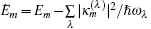

is the operator of nonadiabatic relaxation interaction for transitions between “ phonon-dressed” adiabatic states, with 
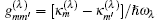

where 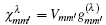
Given the representation of the Hamiltonians (1)– (5), the next step is to establish a hierarchy of fundamental time scales for the dynamics of the density matrix ρ (t) of the whole system following the Liouville– von Neumann quantum evolution equation

We assume that the fastest time in this hierarchy is the adiabatic time at which the state basis of the two parts of the whole system is completely formed so that ρ (t) is factorized by the respective equilibrium density matrix ρ E = exp(− HE/kBT)/trE exp (− HE/kBT) of the E (trace is over the states of the E) and the nonequilibrium density matrix ρ S (t) = trEρ (t) of the S as

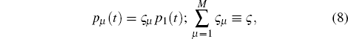
Moreover, for the S, we assume a unique, singled-out metastable state | 0⟩ such that the population pμ (t) = ⟨ μ | ρ S(d) (t)| μ ⟩ of the other states | μ = 1, … , M⟩ is considered to be in quasi-equilibrium represented by only the correspondingly normalized statistical weight ς μ as
where 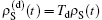

where

is the evolution operator with 
In the above equations,

is the memory kernel having the property of irreversibility 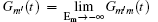

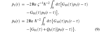
On the other hand, in the limit of much longer times Δ t ≥ τ tr, the evolution of populations (9) is averaged with respect to the stochastic trajectories, thereby assigning the slowest times τ tr ≫ τ st to the occurrence of nonadiabatic relaxation transitions between the two steady-state levels of the S. At the intermediate stationary time Δ t ≈ τ st, any type of relaxation transition between the levels of the S accompanied by creation or annihilation of phonons in the E may occur. Effectively, the adiabatic levels would exhibit a stochastic dynamic characteristic. It is thus needed to carry out an average over the stochastic realizations of populations (9) (usually designated as ⟨ ⟨ … ⟩ ⟩ ), to find the averaged population of aggregated levels, 

In order to correctly follow the aforementioned protocols, one needs to treat the non-Markovianity of integrands in Eq. (9) by providing an explicit average of the involved stochastic functionals ⟨ ⟨ Gmm′ (τ )pm (t − τ )⟩ ⟩ . The situation becomes simpler when random energy level shifts in the S are stationary. In this case, making an average in a transition time scale τ st ≪ Δ t≤ τ tr factorizes the respective quantities on the right-hand side of Eq. (9), for instance, as ⟨ ⟨ f10 (τ )p0 (t − τ )⟩ ⟩ = F10 (τ )P0 (t). This means that in the second-order perturbation theory, the non-Markovianity of metastable level population does not imply itself giving P0 (t − τ ) ≈ P0 (t). Moreover, the stochastically averaged functional

becomes exactly calculable, e.g., for the di- or tri-chotomous stochastic processes and a Gaussian white noise.[22– 27] In such cases, equation (10) reduces to its simplest form

where γ 10 = γ 01 ≡ γ denote the effective level half-width associated with a friction coefficient for the movement of particles within the S when modeled to be open to the E.
Averaging Eq. (9) by using Eqs. (10) and (11) transforms the set of integral differential equations (9) into the system of two ordinary differential equations for nonconserved populations
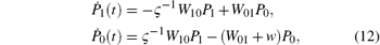
with the following effective transition rate constants (m ≠ m′ = 0, 1) being

It is noteworthy that the transition rate constants in Eq. (13) can be calculated from the Fermi Golden Rule while paying attention not to sum over a dense set of final energy levels of the S but rather to average over stochastic trajectories for transitions having different stationary contributions concentrated in the form of amplitude ς and intensity γ distributions. However, determining the order of carrying out the calculation of Eq. (13) entails some difficulties. At first, one needs to obtain a sum over the number Λ of phonon modes λ = 1, … , Λ , which in general is infinite and may diverge, and only then can the integral over time τ in an interval from 0 to t be evaluated, given ς . In Eqs. (6), (9), (12), and (13), one takes account of random additions to energy levels with the single parameters ς and γ without using the perturbation theory.[23, 24, 25] This allows the analyses of different regimes for transitions dependent on the values of stochastic intensity γ and adiabatic frequency | Ω mm′ | parameters for the S in different limiting cases. Therefore, making necessary assumptions about the relation between these parameters and considering the dependences of nonadiabatic couplings 
We thus note that in tracing a kinetic behavior of the S from its initial (the summary input) to its ultimate (the metastable output) levels, the calculable results are restricted to only two limiting cases of nonadiabatic | Ω mm′ | ≫ γ → + 0 and adiabatic γ ≫ | Ω mm′ | → + 0 transitions. Since the estimate ħ γ ≈ kBT holds for both cases, [26, 27] they correspond to the quantum ħ | Ω mm′ | ≫ kBT and classical ħ | Ω mm′ | ≪ kBT limits of Eq. (13), respectively. However, for practically calculating these limits in Eq. (13), it is quite necessary to know the spectral function 

and using the Heaviside step function θ (x) that is 0 for x < 0 and 1 for x ≥ 0 provides a unified expression for the transition rate constant

Thus, a simple yet plausible classification of the reduced, fluctuating two-level S can be based on quantifying the transition rates in the S in only two limits of mechanistic activationless temperature-independent transitions and Arrhenius’ s activation-like exponentially temperature-dependent transitions. In Eq. (15), these correspond to the case W10 = W01 = J of either the classical limit ħ | Ω 10| → 0 (the lower line) or the highly exoergic quantum limit 

of highly endoergic quantum limit 
Figure 1 shows how such a mathematically simple but physically rigorous calculation of the transition rate constants in Eq. (15) can be carried out from the initial formation and subsequent development of the number and position of energy levels within the S in an adiabatic (ergodic-mixing) scale, a stochastic (stationary dynamic) scale, and a transient (nonadiabatic) time scale. As shown in the figure, at the very short adiabatic time t ≈ τ ad, one can say almost nothing about the number of states of the S as well at the possible position of respective energy levels (the leftmost panel of Fig. 1 with the number of points denoting the states). Nevertheless, at these times there occur ergodic-mixing processes in which the mapping of any subset of energy levels of some number A in the S becomes uniformly distributed in it. With an accuracy of the order τ ad, this allows one to generate a particular nonstationary ergodic super source within the S. Furthermore, at the intermediate stochastic time t ≈ τ st for that source, the total number AN of energy levels can be normalized with respect to the one metastable state such that, by looking at every N subsets of A levels as a single subset from a whole closed fully reversible super set, and one obtains an open, irreversible S having the two levels 1 and 0 of different dimensionalities of d1 = AN = M and d0 = 1 (the middle panel of Fig. 1). Moreover, at the same stochastic time, these two energy levels are characterized by dynamical random fluctuations around the steady-state positions with intensity ħ γ ≈ kBT, far smaller than energy separation between the levels. Finally, at the longest transient time t ≈ τ tr, the microscopically reversible nonadiabatic relaxation transitions between the initial level of dimensionality d1 and the ultimate metastable level of dimensionality 1 as well as a macroscopically irreversible decay of the latter are induced to occur providing the S with its time evolution (the rightmost panel of Fig. 1). Therefore, by studying the dependence of development in time of the population P0 (t) of metastable level 0 in Eq. (12) on all of the characteristic variables involved in the two-level model of the irreversibly damped S, one can uncover a unique possibility to provide a quantitative analysis of the degree of cooperativity of the effective two-level irreversible system with a desired control by tuning the equilibrium d1 = ς and kinetic W01 or w parameters.
 | Fig. 1. Illustration of open system states (points and levels) being distinctly distant in energy from each other (in thermal energy units) and evolving in an adiabatic, a stochastic scale, and a transient time scale (characterized in the text). |
Describing the time evolutions of the population P1 (t) of the input (summary) level and the population P0 (t) of the output (metastable) level of the two-level S requires solving the system (12) which, given ergodic-mixing initial conditions P1 (0) = 1 and P0(0) = 0 well approved at negligible times τ ad ≅ t→ 0, is elementary. We have

where

with α being the running control parameter, α ≡ ς − 1W10 and β ≡ W01.
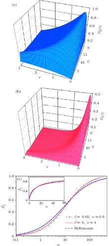
Figure 2 depicts the three-dimensional (3D) behavior of P0 (t) by using two sets of tuned control parameters: β = 6 and w = 4 (a), and β = 0.03 and w = 0.6 (b). For both sets, P0 (t) exhibits bell-shaped variation in time. With an increase in α , it peaks at the maximum 

To describe the degree of cooperativity more quantitatively, one can first consider the odds ratio 
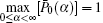

where hα (β , w) is the exponent factor and is a function of the tuned control parameters β and w with α being the running control parameter. This factor is equivalent to the Hill coefficient associated with the cooperativity degree when varying an input rate α leads to a saturable change in 


in the case where level 1 is separated from level 0 by an energy difference Δ E = E1 − E0 ≫ kBT with Δ F = kBT ln (α /β ) being the respective free-energy difference. The latter, according to Δ F = Δ E− kB T ln d1, varies in the infinite interval by correspondingly choosing appropriate values of Δ E and d1 ≥ 1. In log coordinates 
 | Fig. 2. 3D plots of output level population P0(t) versus time and running parameter α for the two sets of tuned parameters β and w (all in inverse time units): (a) β = 6; w = 4 (in red) and (b) β = 0.03; w = 0.6 (in blue); and (c) the corresponding curve fittings of population peaks  |
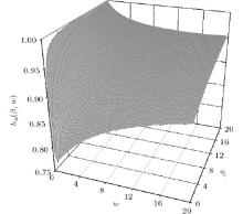
 | Fig. 3. Hill’ s coefficient hα (β , w) (the degree of cooperativity) as a function of tuned β and w, and running α , parameters (in inverse time units). |
To analytically glance at the cooperativity minimum, one sees that in the irreversible case w > 0 at β = 0, from Eq. (16) it follows that P0(t) = [α /(α − w)][exp (− wt)− exp (− α , t)]. In the limit α → w, this expression, represented as P0 (t) = α , t exp [− (α + w)t/2], peaks at time tp = [(α + w)/2]− 1 and approximately yields

The resulting slope of Eq. (19), in the vicinity of α ≈ w, is 1/2e. Therefore, relating this slope to that of Eq. (18) in the vicinity of α ≈ β where hα (β , w) = 1 gives the following bounds for values of the degree of cooperativity

It is worth noticing that the lower limit 2/e ≈ 0.736 of inequality (20) appears to be quite close to the minimum of 0.776 seen in Fig. 3 which validates the consideration. Attaining a greater agreement between numerical and analytical results is, however, difficult, because of numerical errors during the evaluation of hα (β , w) at different β values when varying small values in the vicinity of α ≈ w. It is also important to point out that the choice of the scaling exponent in Eq. (17) does not belong to a unique category, which necessitates considering alternative variants too. A case, for example, would be where the backward rate β is not tuned but running, while the input rate α is tuned instead. For the irreversible two-level S, this implies the use of an enthalpically driven model, within which to achieve a high population of level 0 requires the change of energy difference Δ E between the levels keeping the dimensionality of level 1 constant. Analysis of the corresponding log odds 
In this paper, a kinetic framework for consistently describing the degree of cooperativity of the effective two-level open system (S) weakly coupled to the equilibrium environment (E) in a multiple time scale has been introduced. Quantification of the degree of cooperativity is achieved by associating it with that of the stability affected by the running and tuned controls. To maintain consistency, the kinetic framework rests on tracing the evolution of the S in the three separated time scales: adiabatic, stochastic, and transient, attributed to the characteristic times τ ad, τ st, and τ tr, respectively. In a timescale of τ ad, microscopic structure of the Hamiltonians of the S and the E Eqs. (1)– (3) constrained by the factorization condition (7) for the density matrix of the whole system that evolves according to the Liouville– von Neumann equation (6) is adiabatically formed. At time τ st, a stationary distribution for random fluctuations of position of the energy levels of the S Eq. (10) is stochastically achieved. At time τ tr, averaged probability of transition (13) between the two levels of the S in kinetic equation for level population (12) is established. However, there is a cost to pay to exploit these time scales as one cannot rigorously feature the cooperativity as a controllable one at all times. Instead, one associates it with the degree regarded integrally fixed at times t ≤ τ ad but gradually variable at times t ≥ τ st. Hence, any kinetic framework to quantify the cooperativity needs to be able to take into consideration such special conditions.
In this respect, one can infer several consequences of the use of a kinetic framework in quantifying the degree of cooperativity of the S in a microscopic approach that is worth being remarked on the advantage over other phenomenological approaches. The first consequence is to deal with the idea of the correspondence between stability and cooperativity. Such a relationship is cumbersome to establish due to the poor understanding of kinetics of the S with a multitude of fluctuating energy levels and fundamental difficulties in consistently reducing a complex behavior of such a multi-level S to a much simpler behavior of the two-level S in the different time scales. To circumvent these difficulties, in this work we have used a model of the nonequilibrium S characterized by randomly fluctuating levels which is able to correctly characterize its weak interaction with the equilibrium E, Eqs. (1)– (5), within the microscopic approach.[23, 24, 25, 26, 27] Preference for this approach arises from the possibility to use a unified expression (13) of the averaged rate constant Wmm′ for describing transitions between the two energy levels of different dimensionalities in the framework of kinetic equations for level populations P0, 1 (t) Eq. (12). Knowing a relation of the intensity γ of level fluctuations to the frequency | Ω 10 | of dynamic oscillations in the S gives the corresponding calculus of Wmm′ for the two most important limiting cases of nonadiabatic and adiabatic transitions between widely separated | Ω 10 | ≫ kBT/ħ ≫ γ and nearly degenerate | Ω 10| ≪ γ ≈ kBT/ħ levels, respectively, as Eqs. (14) and (15). Moreover, one can straightforwardly associate these cases with the corresponding quantum and classical limits, and correctly differentiate them between the roles played by enthalpic and entropic factors in the two-level S to guarantee its full stability (associated with the unit cooperativity) and its partial instability (associated with a “ negative” or fractional cooperativity), respectively.
The second consequence is to entail a dependence of the degree of cooperativity on the context in which its value is defined. The context-dependent analysis commonly relates the strengths of nonadditive interactions to their actual contributions to kinetics of the S.[33] On the contrary, we have provided a context-dependence with relating a degree hα (β , w) to controlled parameters β and w by suggesting the statistically weighted distribution (8) for grouping the nearly degenerate levels μ = 1, 2, … , M to a single level 1 of dimensionality d1 = ς , (cf. Eqs. (9) and (12)). We find that this effect could reveal itself only when the input rate α (or, equivalently, the dimensionality d1) is considered as running while the backward β and the output w rates are both tuned (see Fig. 3). It disappears in an otherwise scenario. In such a context, the “ negative” cooperativity of the S might not be enthalpically driven but only entropically driven. This corresponds to the very definition of the stable multi-level S as the one which obeys a microscopic reversibility of enthalpically driven transitions between the energy levels without a change in the entropically driven number of levels.
The third consequence is to be concerned with the limits found for the degree of cooperativity of the two-level S (Eq. (20)). There are two questions one asks about these limits. The first one is whether degree h can be larger than 1 and lower than 2/e. If the answer is affirmative, the second question arises whether it is possible to understand why this is so. Certainly, with respect to the maximum stability of the S, it is a convention to take a maximum degree of cooperativity normalized to unity. Nevertheless, there are many stable multi-level systems, where h < 0.7 and even h ≈ 0.2− 0.3.[34] Yet, in these cases, three-body (or more) processes come into play, leading to the anti-cooperative effects with the very low h.[35] At the same time, the Michaelis– Menten reaction, corresponding to the nonstationary kinetics of the irreversible two-level S, is known as the realization of the mass-action law with any implementation of the cooperative behavior.[11, 12, 36] However, in general, relation (20) points to the emergence of a “ negative” cooperativity just for such an elementary (i.e., the Michaelis– Menten) case. In this regard, the limit (20) has a universal meaning in a sense of pointing to the unstable kinetics of the S.
Finally, the fourth consequence is to refer to the applicability of a kinetic framework proposed to describe the cooperativity of the S viewed here as a natural molecular structure to a wider class of systems including information sources or agencies. It is customary to represent an information agency as a stationary, stable, and ergodic system consisting of many operational units or blocks with multiple feed-forwards and feedbacks.[37] Furthermore, such a system constantly evolves with time owing to the coupling between the units and to the information environment with performing an exchange between energy (material efforts) and matter (particles or information entities). Thus, an agency becomes analogous to the finite-level nonequilibrium S interacting with the infinite-level equilibrium E. By this analogy, one could directly associate the cooperativity of some agency with its stability by quantifying the control of it with a particular degree due to which both the corresponding levels and the respective number of levels are collectively correlated (or cooperatively interact) between each other in order to provide the agency with the desired stable structure. Therefore, it is straightforward to relate the decrease of the degree of cooperativity to the fall in the control of stability, thereby leading to the conclusion that, when normalized, there exist the limits for such a degree Eq. (20), attaining the floor which breaks down the stability. However, this will be the case only if the cooperativity is entropically driven with α being the running input control parameter while the corresponding backward and output control parameters will be tuned to be quite small for β → 0 and nonzero for w > 0, respectively, which are shown in Fig. 3. To regain the controllability, it is sufficient to regularize either of these instabilities by making the backward control nonzero β > 0 or fully cutting off the output control w→ 0. The latter directly relates to neglecting an irreversible kinetic stage in the OS providing it with a well-controlled reversibility.
In a general conclusion, nonstationary irreversible kinetics of the few-level nonequilibrium open system (S) weakly interacting with the equilibrium environment (E) depends on many dynamic factors that can influence both the degree h of cooperativity of the S and its stability. When associated with the reduced case, the effective two-level S becomes a system of the two fluctuating energy levels with two rates of reversible transitions between them and one rate of irreversible decay of some of them (Fig. 1). Dealing with these, we use four independent parameters united in a quadruple {Ω , α , β , w} (Eqs. (14) and (15)). Here Ω ≡ | Ω 10| is the fast absolute frequency of oscillations between the extended energy levels 1 and 0 of the S, α is the reversible input rate, β is the reversible backward rate, and w is the irreversible output rate. To provide the S with a controllable driving of its cooperativity (or stability) to a particular degree hα (β , w), one first sets Ω which is equivalent to fixing β , then runs α with w given and finally plots hα (β , w) as a function of tuned β and w (Eq. (17)). The corresponding 3D graph is depicted in Fig. 3. If w = 0, then the S is almost stable and hence non-cooperative, yet at w > 0 it becomes unstable and “ negatively” cooperative. Thus, to control w is the necessary condition influencing the appearance or the disappearance of cooperativity in the S. The degree of cooperativity depends, however, also on the choice of β . At β → 0, this degree takes its lower limit
| 1 |
|
| 2 |
|
| 3 |
|
| 4 |
|
| 5 |
|
| 6 |
|
| 7 |
|
| 8 |
|
| 9 |
|
| 10 |
|
| 11 |
|
| 12 |
|
| 13 |
|
| 14 |
|
| 15 |
|
| 16 |
|
| 17 |
|
| 18 |
|
| 19 |
|
| 20 |
|
| 21 |
|
| 22 |
|
| 23 |
|
| 24 |
|
| 25 |
|
| 26 |
|
| 27 |
|
| 28 |
|
| 29 |
|
| 30 |
|
| 31 |
|
| 32 |
|
| 33 |
|
| 34 |
|
| 35 |
|
| 36 |
|
| 37 |
|
| 38 |
|
| 39 |
|
| 40 |
|
| 41 |
|