Short-pulse high-power microwave breakdown at high pressures*
[Zhao Peng-Chenga), b) , Liao Chengb)†  , Feng Ju
b) ]
, Feng Ju|
|


Corresponding author. E-mail: c.liao@swjtu.edu.cn
Project supported by the National Basic Research Program of China (Grant No. 2013CB328904), the NSAF of China (Grant No. U1330109), and 2012 Doctoral Innovation Funds of Southwest Jiaotong University.
The fluid model is proposed to investigate the gas breakdown driven by a short-pulse (such as a Gaussian pulse) high-power microwave at high pressures. However, the fluid model requires specification of the electron energy distribution function (EEDF); the common assumption of a Maxwellian EEDF can result in the inaccurate breakdown prediction when the electrons are not in equilibrium. We confirm that the influence of the incident pulse shape on the EEDF is tiny at high pressures by using the particle-in-cell Monte Carlo collision (PIC-MCC) model. As a result, the EEDF for a rectangular microwave pulse directly derived from the Boltzmann equation solver Bolsig+ is introduced into the fluid model for predicting the breakdown threshold of the non-rectangular pulse over a wide range of pressures, and the obtained results are very well matched with those of the PIC-MCC simulations. The time evolution of a non-rectangular pulse breakdown in gas, obtained by the fluid model with the EEDF from Bolsig+, is presented and analyzed at different pressures. In addition, the effect of the incident pulse shape on the gas breakdown is discussed.
The high-power microwave (HPM) has important applications in military and civilian fields, such as directed energy weapons, creation of artificial plasma mirrors, long distance wireless energy transport, and so on.[1] In recent years, the peak electric field of the HPM has reached several MV/m, [2, 3] which is close to or exceeds the gas breakdown threshold at high pressures. Once the gas breakdown occurs, the generated plasma strongly hinders the radiation and propagation of the HPM. Therefore, it is very important to study and understand the HPM breakdown in gas.
The HPM breakdown in gas has been studied by many investigators.[4– 8] These studies focus mainly on the gas breakdown driven by the continuous wave or the rectangular microwave pulses. So far, we know very little about the case of the short pulses, such as the Gaussian pulse, modulated Gaussian pulse, differentiated Gaussian pulses, and fast rise-time pulse, which are often generated in experiments. For example, an L-band magnetically insulated transmission-line oscillator is used as a source to generate the short pulse similar to the modulated Gaussian pulse.[3]
The fluid model has proven to be a key tool for analyzing gas plasma reaction and parameters due to simplicity and speed.[9, 10] In this model, the electron energy distribution function (EEDF), which is an important parameter to calculate transport coefficients (ionization frequency, attachment frequency, collision frequency, and energy loss frequency), was often assumed to be the Maxwellian EEDF. The assumption can lead to inaccurate breakdown prediction when the electrons deviate significantly from equilibrium.[9] A fast method for determining the EEDF in the non-equilibrium is to solve the Boltzmann equation (BE) directly. For example, making use of the two-term approximation, the BE solver Bolsig+ has been developed by Hagelaar and Pitchford, [11] which has a great advantage over the particle-in-cell-Monte Carlo collision (PIC-MCC) method in speed. In our previous work, the EEDF derived from Bolsig+ was introduced into the fluid model to predict the breakdown time of the rectangular microwave pulse, which is very well matched with that of PIC-MCC simulations.[12] However, the EEDF for the non-rectangular microwave pulse, whose knowledge is still scanty, cannot be directly determined by Bolsig+ .
In this paper, to focus on the essential physics, we avoid the complexity of air chemistry, and instead use the noble gas, argon. The influence of the HPM pulse shape on the EEDF is analyzed using the PIC-MCC method, [13, 14] in order to explore whether the EEDF for the rectangular pulse obtained by Bolsig+ can well approximate that for the non-rectangular pulse. Then the EEDF for the rectangular pulse derived from Bolsig+ is introduced into the fluid model to predict the breakdown threshold of the non-rectangular pulse at high pressures, and the obtained results are compared with those of PIC-MCC simulations. Besides, making use of the fluid model with the EEDF from Bolsig+ , we simulate the time evolution of the gas breakdown driven by a non-rectangular pulse, and discuss the effect of the incident pulse shape on the gas breakdown.
The basic equations for the one-dimensional fluid model can be written as follows:[5, 15]


where Ex and Ez represent the electric field components along the x axis and the z axis, Hy is the magnetic component along the y axis, qe and me denote the charge and mass of electron, ε 0 and μ 0 are the permittivity and permeability of free space, the transport coefficients ν i, ν a, ν c, and ν l are the ionization frequency, attachment frequency, collision frequency, and energy loss frequency, Ne denotes the free electron density, and Ux, Uz, and Ue can be written as

In Eq. (8), 


The transport coefficients are important to describe the interaction of neutral molecules (atoms) and the electrons accelerated by the HPM, as shown in Eqs. (4)– (7). The common method for calculating these coefficients is to integrate the collision cross section[16] over the EEDF.[12] For example, the ionization frequency can be defined as

where MAr and NAr are the mass and density of the argon atom, σ ion is the ionization cross section, and f(ε e,
The BE solver Bolsig+ [11] is able to predict the EEDF for a rectangular microwave pulse directly. In order to find the EEDF for non-rectangular pulses, we will check whether it can be well approximated by the EEDF for a rectangular pulse derived from Bolsig+ in the following section, where the one-dimensional PIC-MCC code[13] is employed to predict the ‘ exact’ EEDF, and validate the accuracy of the fluid model with the EEDF from Bolsig+ .
The finite-difference time-domain method has been employed to solve the fluid model numerically.[15] At the initial time, we assume that there are a small number of seed electrons (Ne0 = 1.0 × 10⁶ m− 3) in argon. The simulation domain is five meters. The incident pulse with the polarization along the x axis propagates in the z direction, and its shape is taken to be the rectangular pulse, Gaussian pulse, modulated Gaussian pulse, differentiated Gaussian pulse, and fast rise-time pulse, respectively. These pulses in time can be expressed as follows:


where Ep is the peak value of the pulse, ENor is the normalizing factor for the differentiated Gaussian and fast rise-time pulse, tp is the pulse width of the rectangular pulse, f is the center frequency of the rectangular and modulated Gaussian pulse, t0 = 0.8τ , and α and β are the parameters for adjustment of the shape of the fast rise-time pulse. The width of the non-rectangular pulse is defined as the interval between the leading edge and trailing edge where the amplitude is about a tenth of the peak value. Taking the pulses with a width of 10 ns and a peak value of 1 for example, the parameters controlling the pulse shape are introduced in detail. In this case, tp = 1 × 10− 8 and f = 2.85 × 10⁹ for the rectangular pulse, τ = 1.2 × 10− 8 and t0 = 0.8τ for the Gaussian pulse and modulated Gaussian pulse, ENor = 8.33, τ = 9.09 × 10− 9, and t0 = 0.8τ for the differentiated Gaussian pulse, and ENor = 13.02, α = 4.3 × 10⁸ and β = 5.3 × 10⁸ for the fast rise-time pulse. It should be pointed out that the high-power microwave belongs to the high-frequency oscillating pulses in general, and equations (11), (13), and (14) can only be considered as its envelopes.
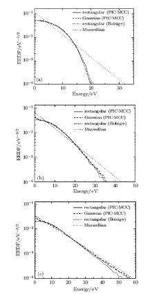
Figure 1 shows the comparison among the EEDFs for the rectangular pulse from PIC-MCC, the EEDF for the Gaussian pulse from PIC-MCC, the EEDF for the rectangular pulse from the BE solver Bolsig+ , and the Maxwellian EEDF. In Fig. 1, the peak value and width of the incident pulse are 3 MV/m and 10 ns (other parameters see Section 2), and the pressure is 500, 100, and 30 Torr (1 Torr = 1.33322 × 10² Pa), respectively. The mean electron energy corresponding to the EEDF shown in Fig. 1 is 6.8 eV for p = 500 Torr, 10 eV for p = 100 Torr, and 15 eV for p = 30 Torr. It is found from the PIC-MCC simulation results that the EEDF for the Gaussian pulse is very similar to that in the rectangular pulse field at the three different pressures. The similar results are also found for other pulses, such as the modulated Gaussian pulse, differentiated Gaussian pulse, and fast rising pulse shown in Eqs. (12)– (14), indicating that the pulse shape has a very small influence on the EEDF. We also see from Fig. 1 that the EEDF for the rectangular pulse directly derived from the BE solver Bolsig+ agree very well with that from the PIC-MCC simulations at the three different pressures. These results above suggest that, at the same mean electron energy, the EEDF for the non-rectangular pulse can be well approximated by the EEDF for the rectangular pulse directly derived from Bolsig+ .
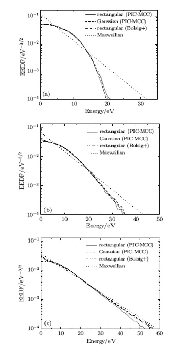 | Fig. 1. EEDF for rectangular pulse from PIC-MCC, EEDF for Gaussian pulse from PIC-MCC, EEDF for rectangular pulse from Bolsig+ and Maxwellian EEDF at (a) 500 Torr, (b) p = 100 Torr, and (c) 30 Torr. |
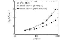
The EEDF for the Gaussian pulse deviates obviously from the Maxwellian distribution at high pressures and intermediate pressures (see Figs. 1(a) and 1(b)), while at low pressures, the two are quite similar (see Fig. 1(c)). The transition of the EEDF from Druyvesteyn[17] at high pressures to the Maxwellian at low pressures can be attributed to the change in electron heating and cooling processes. This suggests also that adopting the Maxwellian distribution in the fluid model can result in inaccurate breakdown prediction at intermediate pressures and high pressures. Taking the Gaussian pulse with the width of 10 ns for example, we present the effect of different EEDFs on the breakdown threshold, as shown in Fig. 2. The breakdown threshold is defined as the peak value of the incident pulse when the electron density reaches 108 times the initial density during the pulse width. The breakdown threshold of the fluid model with the EEDF from Bolsig+ reasonably matches that of PIC-MCC simulations, while the threshold from the Maxwellian EEDF is underestimated at intermediate and high pressures. This is because the high energy tail of the Maxwellian EEDF shown in Figs. 1(a) and 1(b) leads to an overestimation in the ionization frequency.
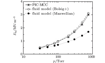 | Fig. 2. Breakdown threshold of Gaussian pulse with the width of 10 ns for PIC-MCC, fluid model with the EEDF from Bolsig+ , and fluid model with Maxwellian EEDF. |
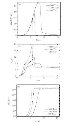
The time evolution of the Gaussian pulse breakdown at three different argon pressures is obtained by the fluid model with the EEDF from Bolsig+ , as shown in Fig. 3. The width and peak of the incident Gaussian pulse are 10 ns and 2.8 MV/m. Once the mean electron energy is high enough to ionize the argon atom, the electron density grows sharply till it reaches a saturation level, as shown in Figs. 3(b) and 3(c). The mean electron energy increases nonlinearly with the electric field, and the variation of the electron density with time follows approximately an exponential distribution. After the argon breakdown occurs, the electron density is limited in a saturation level, which is high enough to attenuate the electron field and mean electron energy significantly, as shown in Figs. 3(a) and 3(b). In other words, it is the tail erosion of the pulse that keeps the electron density from growing.
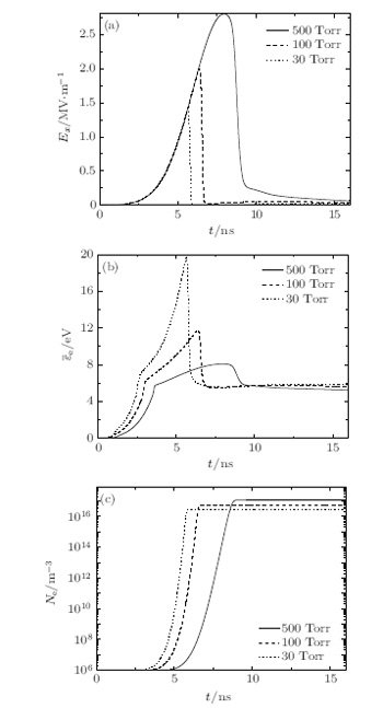 | Fig. 3. Time evolution of Gaussian pulse breakdown in argon at different pressures. (a) Electric field, (b) mean electron energy, and (c) electron density. |
It can also be found from Fig. 3 that, at p = 500 Torr, the mean electron energy is low, and a weak breakdown is generated, i.e., the pulse width is shortened whereas the pulse peak shows little change. With the pressure decreasing (e.g. 100 Torr and 30 Torr), the mean electron energy and the corresponding ν i/NAr increase. Although NAr decreases with the pressure decreasing, the product of NAr and ν i/NAr is found to increase by calculation. As a result, at a lower pressure, the breakdown formation time is shorter, and the attenuation of the pulse tail becomes larger, as shown in Fig. 3. We see also from Fig. 3(c) that the saturation level of electron density decreases with the pressure decreasing. The saturation level of electron density is close to the cut-off plasma density, and the latter can be written as[7]

where ω represents the microwave angular frequency. Since ν c∼ 7 × 10⁹p where p is the pressure in Torr, [15] the cut-off plasma density is found to decrease with p decreasing by Eq. (15). As a result, at a lower pressure, the saturation level of electron density becomes lower, as shown in Fig. 3(c). Although figure 3 is shown only for the Gaussian pulse, the general behavior of the breakdown is observed for other pulses.
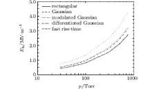
The effect of the microwave pulse shape (see Eqs. (10)– (14)) on the argon breakdown threshold is considered using the fluid model with the EEDF from Bolsig+ , as shown in Fig. 4. Of the breakdown thresholds of these pulses with the width of 10 ns, the modulated Gaussian pulse has the highest one. The breakdown threshold of the Gaussian pulse is approximately equal to that of the fast rise-time pulse, indicating that the influence of the rise time of the pulse on the breakdown threshold is tiny. The differentiated Gaussian pulse can be considered as a rectangular pulse with a very low frequency, and therefore it has a breakdown threshold approximately equal to that of the rectangular pulse.
 | Fig. 4. Breakdown thresholds of rectangular, Gaussian, modulated Gaussian, differentiated Gaussian, and fast rise-time pulses with the width of 10 ns. |
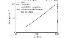
At the fixed pulse width of 10 ns, the maximum or critical transmitted pulse energy fluences, in J/m2, are predicted for the different pulses when no breakdown occurs, as shown in Fig. 5. In this case, the pulse peak should be equal to the breakdown threshold shown in Fig. 4. The energy fluence can be calculated by 
 | Fig. 5. Critical energy fluences in argon for rectangular, Gaussian, modulated Gaussian, differentiated Gaussian, and fast rise-time pulses with the width of 10 ns. |
The fluid model has been extended for application to the non-rectangular HPM pulse breakdown in argon at high pressures. The fluid model is compared with PIC-MCC, showing similar predictions for the breakdown threshold of the non-rectangular pulse, i.e., the Gaussian pulse, when adopting the EEDF for a rectangular pulse derived from the BE solver Bolsig+ . This is because the pulse shape has a very small influence on the EEDF under the same mean electron energy. We also confirm that the Maxwellian EEDF leads to the poor breakdown prediction for the non-rectangular pulse, when electrons deviate obviously from equilibrium, for example at high argon pressures. Taking the Gaussian pulse for example, we present and analyze the time evolution of the breakdown at different pressures. Although the effect of the incident pulse shape on the breakdown threshold is obvious, the critical energy fluences of different pulses under the case of the pulse peak equal to the breakdown threshold are approximately equal. The fluid model with the EEDF derived from Bolsig+ can also be used to predict the breakdown of other short pulses without those considered in this paper, and in other background gases, such as air, nitrogen, sulphur hexafluoride, and so on.
| 1 |
|
| 2 |
|
| 3 |
|
| 4 |
|
| 5 |
|
| 6 |
|
| 7 |
|
| 8 |
|
| 9 |
|
| 10 |
|
| 11 |
|
| 12 |
|
| 13 |
|
| 14 |
|
| 15 |
|
| 16 |
|
| 17 |
|