Global observation of wind and temperature profiles of the mid-atmosphere is a basis of research on the atmospheric dynamics and forecasting the future evolution of the atmosphere. The Doppler wind lidar is superior in terms of good accuracy and high spatial resolution when compared with other methods. Wind measurements of the mid-atmosphere are still rarely reported. Within this height range, the Mie signal, which can be used in lower atmosphere with high frequency accuracy, is weak, and this height is usually beyond the access of balloons and radar. A Rayleigh Doppler lidar is a reliable way to cover this height range. The other methods, such as rockets, have poor time and region coverage.^[1] Although a space-borne DWL is a potential way to realize observations within this range, it is still under schedule.^{[2– 5]}

Doppler wind lidars (DWLs) can be divided into two types: a coherent and an incoherent (or direct) method. With the coherent method, the Doppler shift is obtained by beating the narrowband Mie backscatter with a local continuous-wave laser; ^{[6, 7]} with the incoherent method, the Doppler shift can be measured directly by a frequency discriminator, such as Fabry– Perot interferometer, ^{[8– 16]} iodine absorption filter, ^[17] Fizzeau interferometer, ^[18] Mach-Zehnder interferometer, ^[19] and Michelson interferometer.^[20] The Rayleigh Doppler Wind Lidar (RDWL) takes advantage of the temperature-dependent Rayleigh backscatter. Mie backscatter is weak at heights above 15  km away from ground. However, the separation of Mie and Rayleigh component is necessary to reach a higher accuracy.^[21] Although the Brillouin effect is significant at low altitudes, the Brillouin effect on the backscatter spectrum is weak at heights above 15  km from ground.^[22]

Given that temperature has a broadening effect on the Rayleigh spectrum, temperature influence should be taken into account during wind retrieval. Errors of temperature profiles will lead to errors of wind that cannot be ignored.^[23] Simultaneous observations of temperature and wind are critical for accurate correction of the wind from temperature influence.

The rest of this paper is organized as follows. In Section  2, the double-edge RDWL theory is reviewed. In Section  3, the wind errors caused by the temperature influence are discussed in detail. In Section  4, the error of the integrating technique is discussed and the observations of temperature are presented. In Section  5, the correction process of wind retrieval from the temperature influence is introduced and the corrected wind profile is also shown.

The double-edge technique is employed with a higher measurement accuracy of the Doppler-shift of the atmosphere backscatter than the original edge technique. In this lidar system, a triple channel Fabry– Perot interferometer (FPI) with two signal channels and one lock channel is used to detect the Doppler shift of the backscatter and the frequency of the outgoing laser, respectively. Three channels have the same parameters, except for the cavity spacing, which determine the central frequency of the transmission curve. As a result, the transmission curves of two signal channels intersect at the position of the edge where the sensitivity of the Rayleigh component is equal to the sensitivity of the Mie component. At the same time, the crosspoint of two signal channels is located at half the maximum of the lock channel, leading to the highest locking precision and the largest dynamic range. As a result, the frequency of the outgoing laser can be locked at the crosspoint of the two signal channels by detecting the transmission of the lock channel. Considering the same sensitivity of the Rayleigh and Mie components at the crosspoint and the reduction of the aerosol above 15  km, only Rayleigh scattering is considered during the wind retrieval.

On average, air molecules move with the wind, so the line of sight (LOS) wind velocity can be obtained from the Doppler shift of the Rayleigh backscatter. However, with a Doppler shift proportional to the LOS wind velocity, the spectrum of the Rayleigh backscatter is broadened due to random motions of the air molecules caused by thermal agitation and collisions. For air molecules, thermal agitation accounts for the primary cause of the broadening. The spectrum of the Rayleigh backscatter is given by a Gauss function as

where Δ ν _R is the full width at half maximum (FWHM) of the Rayleigh backscatter spectrum and is given by

where k is the Boltzmann constant, T_a is the temperature of the atmosphere, λ is the wavelength of the outgoing laser, and M is the average mass of one single air molecule. The transmission curve of the FPI signal channel is written as

where B is the background constant, T_pe is the peak value of the transmission curve, R_e is the effective reflectivity, Δ ν _FSR is the FSR of the FPI, θ ₀ is the half-maximum divergence of the collimated beams to the FPI, ν ₀ is the frequency of the outgoing laser, and ν _c is the central frequency of the transmission curve. The transmission curves of the two signal channels H_i (ν ) (i = 1, 2) are fitted during the calibration procedure. Thus, the transmission of the Rayleigh backscatter is a convolution of the FPI transmission H_i (ν ), the Rayleigh spectrum f_R (ν , T), and the outgoing laser spectrum f_L(ν ), and is written as

The spectrum of the laser is given by a Gauss function as

where Δ ν _L is the FWHM of the laser spectrum. Using Eqs.  (1), (3), and (5), the convolution result of Eq. (4) can be deduced as

where .^[24] The theoretical derivation of this convolution and the development of H(ν ) are beyond the scope of this paper and will be introduced elsewhere. The response function is then defined as

When considering the influence of temperature on the spectrum of the Rayleigh backscatter, the Rayleigh response is a function of the Doppler shift and temperature. Using Eq.  (7), the Doppler shift ν _D can be derived from the photon counts N₁ and N₂ of two signal channels. After that, LOS wind can be calculated from the Doppler shift based on the Doppler formula

However, different values of the temperature bring different relations between response and Doppler shift, which means that an exact response from observation leads to different Doppler shifts under different temperatures. Thus, how temperature influences the wind inversion is worth discussing.

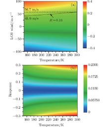
At a specific temperature, the response function given by Eq.  (7) turns into a curve relating the Doppler shift ν _D to the Rayleigh response R. This curve is nearly a straight line. However, the slope of this curve changes as temperature changes.^[23] Values of the response are plotted as a function of temperature and LOS wind (or Doppler shift) in Fig.  1(a). As shown by the black line in this figure, the same value of response (R = 0.16, corresponding to LOS wind about 50  m/s) leads to different LOS winds when temperature changes. As temperature changes from 150  K to 300  K, LOS wind varies from 41.6  m/s to 56.7  m/s, which means that a 10-K interval leads to an LOS wind change of about 1  m/s (corresponding to 2% error of the LOS wind). The wind error caused by 1-K temperature change is plotted as a function of temperature and response in Fig.  1(b). A 1-K error of temperature leads to a relative error of about 0.2% of the LOS wind (error of 0.1  m/s at LOS wind of 50  m/s) at maximum. Compared with the designed system accuracy requirement, the temperature which is introduced into the wind inversion must have an accuracy of a few K. The temperature profiles from numerical prediction system or atmosphere models can hardly meet this requirement. A real-time accurate temperature observation at the same place is necessary during the wind observation. The temperature profiles obtained from this lidar observation and their accuracy analysis are introduced in detail in Section  4.

Fig.  1.

	Figure Option ViewDownloadNew Window
	Fig.  1. (a) Values of the response as a function of temperature and LOS wind; (b) wind error caused by 1-K temperature change as a function of temperature and response.

When calculating the errors of the LOS wind caused by the uncertainty of the temperature, the actual parameters of the FPIs of this lidar system are used. These parameters are obtained in the calibration process. The transmission curves of the FPI are obtained by scanning the length of the FPI cavity. The transmission curves of the FPI are then fitted using the mathematical model as shown by Eq.  (3). After which, the parameters obtained from the fitting procedure are substituted into Eqs.  (6) and (7) to calculate the response function, which is function of temperature and Doppler shift. Finally, the temperature-wind map of response value and the temperature-response map of LOS wind errors are calculated based on the response function. Thus, the parameters of the FPI obtained from the calibration process influence the result of the error analysis to a great degree. It is worthwhile noting that the reflectivity R_e is a parameter that determines the FWHM of the transmission curve of the FPI, yielding

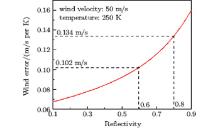
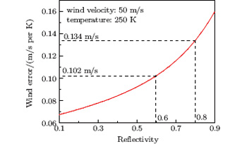
where c is the velocity of light, n is the index of refraction, l is the length of the FPI cavity. A change of Δ ν leads to a change of the slope of the response curve, and the LOS wind error of 1-K temperature uncertainty changes accordingly. The LOS wind error of 1-K temperature uncertainty versus reflectivity is shown in Fig.  2. A higher reflectivity leads to a higher error of wind. As reflectivity changes from 0.6 to 0.8, the error of wind grows from 0.102  m/s to 0.134  m/s, corresponding to an error increase of 31%. Therefore, this considerable error increase with higher value of reflectivity is worth taking into account when designing the FPI.

Fig.  2.

	Figure Option ViewDownloadNew Window
	Fig.  2. LOS wind errors of 1-K temperature uncertainty versus reflectivity. As reflectivity changes from 0.6 to 0.8, the error of wind grows from 0.102  m/s to 0.134  m/s, corresponding to an error increase of 31%.

The temperature profiles are derived from the raw data of the temperature channel by using integration technique.^[25] Taking advantage of the lidar equation, the spatial density N(z) of atmospheric molecules relative to the reference altitude can be derived from the elastic lidar return signal S(z) as

where τ (z_ref, z) is the atmospheric transmission between the reference altitude z_ref and the measurement height z, N(z_ref) is the spatial density of atmospheric molecules at the reference altitude, S(z) and S(z_ref) are the elastic lidar return signals at the measurement height and the reference height, respectively, and z₀ is the altitude of the lidar above sea level. By making use of the ideal-gas law, the temperature profile can be derived from N(z) as

where g is the acceleration of gravity. Thus, with the input of N(z_ref) and T(z_ref), the temperature profile can be derived in successive steps, starting from the reference height. CIRA 86 model^[26] is used for the reference temperature and density. The variance of the temperature is given by

where SNR(z) and SNR(z_ref) are the signal-to-noise ratios, which are inversely proportional to the square root of the photon counts of the detector at altitudes z₀ and z_ref, respectively; Q(z) and Q(z_ref) are the photon counts of the backscatters at z₀ and z_ref, respectively; and, L is the normalization constant.

Fig.  3.

	Figure Option ViewDownloadNew Window
	Fig.  3. Typical raw data from the temperature measurements. An accumulating time of 30  min is adopted and the spatial resolution changes from 200  m to 1  km above 43  km (see the dotted curve).

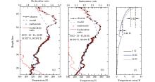
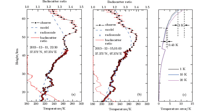
Typical raw data from the temperature measurements are represented in Fig.  3. An accumulating time of 30  min is adopted and the spatial resolution changes from 200  m to 1  km above 43  km, as shown by the dotted curve. Equation  (12) demonstrates a good convergence of this integration technique^[27] when integrating from the reference height to the bottom because the signal reduces exponentially from top to bottom, as shown in Fig.  3. The standard error of the temperature versus height is calculated using Eq.  (12), as shown in Fig.  4(c). From this figure it follows that the temperature error reduces exponentially with the down-ward integration, which is mainly affected by the exponential reducing of signal Q(z). Different temperature standard errors ranging from 1  K to 20  K at reference height lead to a 3-K difference in temperature error at 65  km, and a 0.43-K difference at 55  km. Although the accuracy of the reference-height value is not as significant to the temperature error as that of the photon counts Q(z), as discussed above, the value at the reference height should be much closer to the actual value than this worst-case error analysis, so the error of the integration should be considerably smaller. It should be noted that the jump of the error curve at 43  km in Fig.  4(c) is caused by the change in spatial resolution.

Our observation was performed in Delhi (37.371° N, 97.374° E), northwest of China, throughout December 2013. In order to verify the performance of our lidar, comparison with the radiosonde was made every morning and nightfall if the weather condition permitted observation. The two temperature profiles obtained from December  11 and December  15 observations are compared with the CIRA 86 model and the radiosonde data, which are shown in Figs.  4(a) and 4(b). The error bars indicated in these two figures are calculated on the assumption that the error of the reference-height temperature is 15  K. The observed temperature profiles have good agreement with the radiosonde data above 25  km. However, the temperature deviation occurs below 25  km, and the deviation increases as height decreases, as shown in Fig.  4. We find that, after processing all of the raw data, these are not exceptional events. The reason for these deviations is investigated.

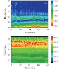
Our temperature retrievals are performed on the assumption that the mesosphere and upper stratosphere are aerosol-free. However, there are possibilities that the aerosol layer might extend above 20  km.^[28] Temperature retrievals from the Rayleigh backscatter are affected by the existence of aerosols because the backscatter will not be proportional to the molecular density of the atmosphere if aerosols exist. Therefore, the deviation of the temperature might be caused by the presence of aerosols. To make sure that aerosols exists in this height range, the backscatter ratio (the ratio of the sum of the scattering cross sections of molecule and aerosol to the scattering cross section of molecule) is calculated from the raw data of the return signal by using the Fernald method.^[29] The profiles of backscatter ratio are shown in Fig.  4. The result shows that aerosols appear at heights below 30 km and increase rapidly downward. Hence, the deviation of the temperature is mainly caused by the presence of aerosols. Therefore, the temperature observation is not reliable at heights below 30 km, owing to the influence of aerosols. The backscatter ratio map of continuous observation from 22:40 December 10 to 01:35 December 11 2013, as shown in Fig.  5(a), confirms the existence of aerosols at heights below 30  km. Figure  5(b) shows the temperature map during the same period. Below the dashed line, the temperature observation is not accurate.

Fig.  4.

Figure Option ViewDownloadNew Window

Fig.  4. (a) A typical temperature profile and backscatter ratio obtained from the raw data on December 11 2013. (b) A typical temperature profile and the backscatter ratio obtained from the raw data on December 15 2013. (c) Standard error of the temperature versus height, different temperature standard errors from 1 K, 10 K, and 20 K at reference heights lead to 3 K difference in temperature error at 65 km, and 0.43 K difference at 55 km.

Fig.  5.

	Figure Option ViewDownloadNew Window
	Fig.  5. (a) Backscatter ratio map and (b) temperature map of continuous observation from 22:40 December 10 to 01:35 December 11 2013.

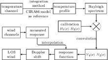
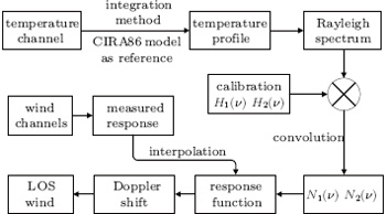
As noted in Section  1, the Brillouin effect is not taken into account during the wind inversion. We also assume that Rayleigh backscatter suffers no contamination by Mie during the wind retrieval. Only the temperature-affected Rayleigh spectrum participates in the wind inversion. As introduced in Section  4, the temperature is calculated from the Rayleigh backscatter, using the integration technique, and the CIRA 86 model is used for reference data. Rayleigh broadening at every interval from the temperature influence is calculated by using the temperature profile from the earlier inversion step, as shown in Eqs.  (1) and (2). It should be noted that we use the temperature data of the radiosonde at heights below 30  km because the observed temperature of the lidar is not reliable below 30  km. The photon counts N_i (ν ) of the Rayleigh return are calculated from the convolution of the FPI transmission curves and the broadened Rayleigh spectrum. According to Eq.  (7), the response function of temperature and Doppler shift is calculated and saved. Using the observed temperature profile, the response function turns into a function of height and Doppler shift. After the actual value of the response at every height interval is measured from the wind channels, a Doppler shift is acquired by interpolation of the measured response to the response function, which is calculated and saved during the earlier step. LOS wind is calculated from the Doppler shift according to Eq.  (8). Figure  6 is a schematic diagram showing how the LOS wind is inverted from the photon counts of the Rayleigh return of the FPI channels.

Fig.  6.

	Figure Option ViewDownloadNew Window
	Fig.  6. Schematic diagram showing how the LOS wind is inverted from the photon counts of the Rayleigh return of the FPI channels and how the wind is corrected from the temperature influence.

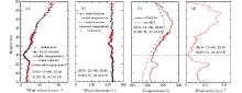
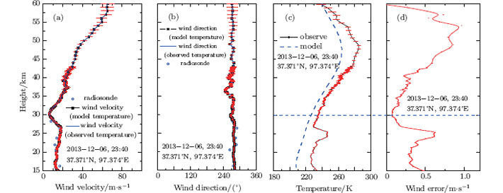
Figures  7(a) and 7(b) show a wind profile and a direction profile measured by our lidar, corrected from the temperature influence. The profiles show that they are in good agreement with the radiosonde data. Wind corrected by the observed temperature (line) is compared with the wind corrected by the model temperature (dotted line). These two profiles, using different temperature data, nearly coincide. However, deviations less than 1-m/s happen between the winds corrected from two different kinds of temperature data. The deviations are shown in Fig.  7(d), and the model temperature and observed temperature used during the correction are shown in Fig.  7(c). The wind deviation, mainly determined by the LOS wind, and the difference between model temperature and observed temperature, is in good agreement with the error analysis in Section  3. In the actual process of wind retrieval, the temperature data from radiosondes are used below 30-km instead of temperature observed by lidar (below the blue dashed line). Although the deviations seem insignificant, a less than 1-m/s error elimination is helpful to improve the system accuracy.

Fig.  7.

Figure Option ViewDownloadNew Window

Fig.  7. (a) A wind profile measured by our lidar and corrected from the temperature influence, compared with the radiosonde data. (b) The wind direction of this wind profile, compared with the radiosonde data. (c) The model and observed temperature profiles used in the wind retrieval. (d) The wind error caused by the difference between the temperature calculated from the model and the temperature observed experimentally.

A mobile Rayleigh Doppler lidar based on double-edge technique is successfully implemented for simultaneously observing wind and temperature at heights 15  km– 60  km away from ground. An analysis of the temperature influence on the wind retrieval is carried out, and the result shows that the temperature broadening of the Rayleigh return spectrum cannot be ignored during the wind inversion. Thus, a simultaneous and accurate observation of temperature during the wind observation is needed. The temperature observation of our lidar has a satisfactory accuracy and precision at heights above 30  km. However, the observed temperature is not reliable at heights below 30  km because of the influence by the presence of aerosol. Therefore, radiosonde data are used at heights below 30-km instead of the observed temperature of the lidar during the wind retrieval. After the correction of the wind from the temperature influence, the wind profiles show good agreement with wind observations from other techniques, demonstrating that the temperature influence on the wind retrieval is correctly treated.

In our future work, long-term and simultaneous observations of temperature and wind will be performed to demonstrate the reliability and stability of this correcting method of wind from temperature influence. An independent aerosol system will be employed to obtain backscatter ratio profiles in order to correct the temperature profiles that are affected by the presence of aerosol at heights below 30  km. At the same time, contamination by Mie will be investigated and considered during the wind retrieval. A rotational Raman lidar will be employed to cover troposphere and lower stratosphere temperature observation because the Rayleigh lidar is seriously affected by aerosol in this range. The emission and receiving efficiency of the system will be improved to reach 80  km in height, reaching the height range (from 80  km to 105  km) of the narrowband sodium lidar developed at the University of Science and Technology of China.^[30] The observation data from this narrowband sodium lidar will then be used as reference data of the integration technique, which is employed during temperature retrieval.