


Comparison of two absorption imaging methods to detect cold atoms in magnetic trap*
[Wang Yan, Hu Zhao-Hui† , Qi Lu]
, Qi Lu]
|
|


Corresponding author. E-mail: huzh@buaa.edu.cn
Project supported by the National Natural Science Foundation of China (Grant Nos. 61227902 and 61121003) and the National Defense Basic Scientific Research Program of China (Grant No. B2120132005).
Two methods of absorption imaging to detect cold atoms in a magnetic trap are implemented for a high-precision cold atom interferometer. In the first method, a probe laser which is in resonance with a cycle transition frequency is used to evaluate the quantity and distribution of the atom sample. In the second method, the probe laser is tuned to an open transition frequency, which stimulates a few and constant number of photons per atom. This method has a shorter interaction time and results in absorption images which are not affected by the magnetic field and the light field. We make a comparison of performance between these two imaging methods in the sense of parameters such as pulse duration, light intensity, and magnetic field strength. The experimental results show that the second method is more reliable when detecting the quantity and density profiles of the atoms. These results fit well to the theoretical analysis.
The investigations of cold atom interferometry[1] are of great importance and interest in many applications, such as the highest precision atomic clock, [2] geophysical tests of general relativity, [3] and measurements for navigation.[4] As the basic part of these researches and applications, obtaining of the quantity and distribution of the cold atom cloud is critical and essential. One of the most common methods to image cold atoms is absorption imaging.[5] A typical configuration of the absorption imaging method is to apply a tuned probe laser to a closed-channel cycling transition, [6] which makes the atoms emit photons continuously in the detection period. Although a high signal-to-noise ratio can be reached by using this method, the inhomogeneous probe light density and the disturbed quantization axis affect the scattering rate of the atoms strongly in some applications with a high gradient magnetic field.[7, 8] Thus, this imaging method can be used only to evaluate the approximate quantity of the atom sample and is less reliable in extracting the exact quantity and the distribution of the atom cloud. One method to solve this problem is to switch off the magnetic field during the imaging period. However, the magnetically confined atoms are disturbed in the process of switching and the images result in distortion and deformation.[9, 10] Another absorption imaging method relies on the optical pumping principle of atoms and uses an open-channel transition probe laser. This method has a uniform photon number yielded by each atom and, therefore, it is also insensitive to the magnetic field and the probe light density. Consequently, it achieves much more reliable results for the atom quantity and distribution.
In this paper, we perform these two imaging methods to detect the cold cesium atoms in a magnetic trap region. The rest of this paper is organized as follows. In Section 2 the theoretical analysis and calculations are represented. In Section 3 the experimental setup is described. In Section 4 the experimental results are presented and discussed. The quantity and precise distribution of the atom cloud are obtained by optimizing the imaging parameters.
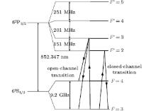
Figure 1 shows the level diagram of cesium D2 line transitions, [11] which is used for imaging. Atoms in the magnetic trap are initially pumped into the F = 3 ground level before imaging. The two probe lasers used in this system are in resonance with F = 3 → F′ = 2 and F = 3 → F′ = 3 transitions.
The first method of absorption imaging is based on the closed-channel transition of F = 3 → F′ = 2.[12] According to the selection rule, [13, 14] the atoms in the F′ = 2 level can only return to the F = 3 level by spontaneously emitting a photon. Consequently, the atoms cycle between F = 3 and F′ = 2 levels during the closed-channel probe pulse, scattering photons continuously. Thus, the scattering rate can be used to estimate the photons scattered by the atoms. The scattering rate is described by the following equation:
where Γ is the natural decay rate (32.89 MHz) of the D2 excited state, Δ is the laser detune, I is the beam intensity, and Isat is the saturation intensity.[10] In this case, Isat is 4.65 mW/cm2 for the F = 3 → F′ = 2 transition and the scattering rate is 8.225 MHz at a saturation intensity.[15] According to the momentum conservation law, the scattering rate (8.225 MHz) corresponds to an average acceleration of 2.9 × 10⁴ m/s2 for a single atom. Assuming that an atom starts from rest, its displacement in detection pulse duration of 50 μ s is about 37.5 μ m, which cannot be neglected compared with the diameter of the atom cloud (about 300 μ m). Since the movements of the atoms are random, the density profiles recorded by the images are not the actual distribution of the atom cloud in the initial time. The displacements of the atoms cause diffusion and distortion in the extracted distribution images. On the other hand, the scattering rate is sensitive to the probe light intensity, the disturbed magnetic quantization axis, and the Zeeman level splitting effect.[16] Therefore, the photon numbers scattered by each atom at different positions are strongly different from each other, resulting in unreliable results. However, the high number of photons leads to a higher signal-to-noise ratio.[17]
 | Fig. 1. Cesium D2 transition hyperfine structure and the optical transitions used for imaging. |
The second method is the open-channel transition method, whose probe laser frequency is in resonance with the F = 3 → F′ = 3 transition. The atoms in F′ = 3 excited state may decay to F = 3 or F = 4 ground state with different probabilities. When atoms decay to the F = 3 ground state, the scattering process repeats again. When atoms decay to the F = 4 ground state, they cease to scatter any photon because the probe laser is 9.2 GHz red-detuned from the F = 4 → F′ = 3 transition. Each of the magnetically trapped atoms in the F = 3 ground state scatters very few photons before being optically pumped to the F = 4 ground state. Such few photons induce a very small displacement that hardly disturbs the magnetic quantization axis. This characteristic also makes the open-channel method insensitive to the density distribution of the probe laser.[18] Most laser beams do not have an absolutely homogeneous density distribution even for the ideal flattened beam.[19] However, no matter how different the beam densities that an atom feels are, it only scatters a few photons averagely in the probe duration. The interaction time is extremely short, so that the absorption process ends quickly, therefore the subsequent variations of the atom cloud are not recorded by the images. To sum up, the open-channel method is more reliable to obtain the accurate quantity and distribution of the atom cloud. The interacting photon number is analyzed below.
The average number of the scattered photons is calculated with two approximations. Firstly, the transition to F′ = 2 or F′ = 4 excited state is ignored by choosing a pulse duration shorter than 50 μ s. This approximation is based on the large detuning between the transition and the probe laser frequency.[20] According to Eq. (1), the scattering rate of the F = 3 → F′ = 3 transition is 8.225 MHz at saturation intensity, while that of the F = 3 → F′ = 2 transition (Δ = 151 MHz) is just about one percent. This means that if the duration of the pulse is short enough, then the transitions to F′ = 2 and F′ = 4 can be neglected. Secondly, because of few interacting photons, the atom cloud is bounded well in the center of the magnetic trap, where the magnetic field strength is almost zero. In addition, the atoms have less displacements during the short interaction time and the influence of Zeeman level shifts can be neglected.[21]
The average interacting photon number can be calculated by summing over the transition probabilities. The relative strength of the transitions of F′ = 3 → F = 3 and F′ = 3 → F = 4 is characterized by the dipole matrix elements. Considering an atom as a two-level system, the effective dipole moment is given by

where ⟨ J||er||J′ ⟩ is the D2 (62S1/2 → 62S3/2) transition dipole matrix element

and SFF′ is the symmetry factor. The relative strength ratio of F = 3 → F′ = 3 transition and F = 3 → F′ = 4 transition is S33/S43 = 27/7 (S33 = 3/8, S43 = 7/72). Thus the probabilities of F′ = 3 → F = 3 transition and F′ = 3 → F = 4 transition are 27/34 and 7/34, as shown in Table 1.[11]
Therefore, the probability P(n) that an atom scatters n photons while being transferred into the F = 4 ground state is P(n) = (7/34)(27/34)n – 1. The average photon number is expected to be
The open-channel method scatters few photons and the absorption process ends very quickly. Thus, the images can record the quantity and distribution information about the atom cloud at the very initial moment.
| Table 1. Cesium D2 transition hyperfine structure and the optical transitions used for imaging. |
The image system is schematically shown in Fig. 2. The distance from the lens to the atoms and that from the lens to the CCD camera are both 300 mm. The typical imaging period includes four steps. First, the optimized double-MOT system (where MOT stands for magnetic optical trap) takes 200 ms to get the cold atoms ready. Second, the current of magnetic coils in the MOT system is adjusted to compress the atoms and load them into the magnetic trap. Then, during the last 3 ms of the loading operation, the cooling laser of the MOT (12 MHz red-detuned from the F = 3 → F′ = 4 hyperfine transition) is extinguished, so that all of the atoms are pumped to the F = 3 ground state by the re-pumping laser (resonant with F = 3 → F′ = 4 hyperfine transition). Finally, at 20 ms after shutting all the lasers of the MOT, the CCD camera and the probe laser are triggered to take an image. The whole process is controlled by a LabVIEW program through an NI 6733 analog output device. All of the lasers in this system are operated by acoustic optical modulators (AOMs) to achieve the frequency shifts.
 | Fig. 2. Absorption imaging configuration. Some photons of the probe light are scattered by the atoms and the shadow created by the “ missing photons” is imaged. The output diameter of the fiber collimator is 4 mm. |
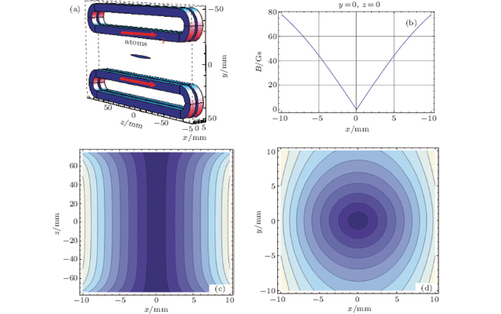 | Fig. 3. (a) The magnetic coils structure; (b) magnetic field versus x; (c) contour plot of magnetic field in plane xz; and, (d) contour plot of magnetic field in plane xy. The simulation is calculated with a current of 35 A. 1 Gs = 10– 4 T. |
The elongated atom cloud is bounded in the center of the magnetic trap, and the trap is generated by a quadrupole coil. The magnetic coil structure and field strength distribution are shown in Fig. 3. In the experiment, a current I = 35 A provides a field gradient of 80 Gs/cm (1 Gs = 10– 4 T) along the x axis and a depth of ≈ 4 mK for the | F = 3, mF = − 3⟩ ground state of cesium. The magnetically confined atoms are located along the z axis at the symmetry axis of the coil.
The images record the atom cloud shadow created by the scattered photons. The original shadow image is subtracted from the background image to obtain the absorption image, which represents the distribution of the atom cloud. Figures 4(a) and 4(b) show the absorption images of the atom cloud achieved by the two respective methods. To compare the images of the two methods under the unified standard, the same background image is used to normalize the intensities of the absorption images. ‘ 1’ represents the intensity of the background laser.
 | Fig. 4. Absorption images taken by (a) the closed-channel transition method and (b) the open-channel transition method. Their intensities are both normalized by the same background image intensity. |
From Fig. 4 it can be seen that the atoms spread more widely in the image taken by closed-channel method than by the open-channel and more photons are absorbed, which is indicated by the fact that the atom spot is brighter in the closed-channel image. In the following parts, the influence of different parameters, such as the pulse duration, the light intensity, the magnetic field strength, and the homogeneity of the probe light, will be studied.
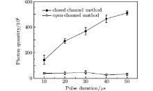
The pulse duration is set to be from 10 μ s to 50 μ s to compare the photon quantity imaged by the two methods. The probe light intensity is half of the saturation intensity here. As shown in Fig. 5, in the open-channel transition method the photon quantity hardly changes when the pulse duration varies, while the photon quantity increases linearly as duration increases in the closed-channel method. Besides, the photon quantity is much more than the open-channel method. It demonstrates that fewer photons are absorbed and the interaction time is very short for the open-channel method, while the absorption process lasts in the whole pulse duration and many more photons are absorbed with the closed-channel method. Broadly speaking, the image results of the open-channel method are independent of the pulse duration while the image results of the closed-channel method are not.
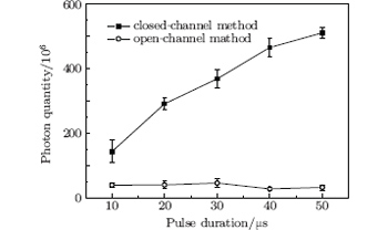 | Fig. 5. Variations of photon quantity with pulse duration obtained by the two methods. |
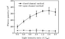
In this subsection, the light intensity is varied to compare the two methods when the intensity is changed from 0.4Isat to 1.6Isat, as shown in Fig. 6. For the open-channel method, the interaction photons are weak and their number is well maintained with the varying light intensity. However, for the closed-channel method, the photon quantity increases linearly with light intensity increase when the intensity is less than 1.2Isat. After the light becomes stronger than 1.2Isat, the photon quantity is nearly stable since the absorption is saturated. The experimental result fits well to Eq. (1). As a result, the open-channel method is not affected by the light intensity while the closed-method is indeed affected by the light intensity.
 | Fig. 6. Variations of photon quantity with light intensity ratio for the two methods. |
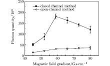
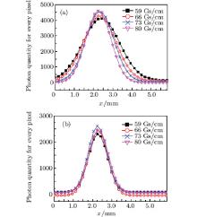
Since the atoms are bounded in the magnetic trap, the influence of the magnetic field variation is studied. For the closed-channel method, the atoms spread out of the central part of the magnetic trap which has near-zero magnetic field strength in the pulse duration, so the Zeeman shift cannot be ignored, especially for the margin of the atom cloud. The Zeeman shift becomes large while the magnetic field strength increases, which leads to the decline of the scattering rate. Thus the photon quantity decreases and the width of the atom cloud narrows down when the magnetic field gradient varies from 60 Gs/cm to 80 Gs/cm, as shown in Figs. 7 and 8(a). When the magnetic field gradient varies from 45 Gs/cm to 60 Gs/cm, the weaker magnetic field traps fewer atoms, the photon quantity rises with the magnetic field gradient increase. After the magnetic field gradient reaches 60 Gs/cm, almost all of the atoms are trapped and the number of the atoms stabilizes.
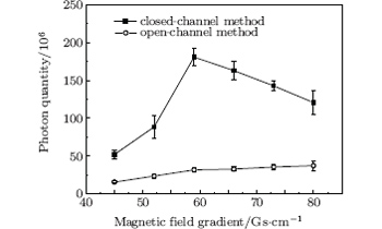 | Fig. 7. Variations of photon quantity with magnetic field gradient, obtained by the two methods. |
For the open-channel method, the situation is similar to the closed-channel method from 45 Gs/cm to 60 Gs/cm. The number of atoms is unstable and the photon quantity is increasing. However, when the magnetic field gradient is stronger than 60 Gs/cm, the photon quantity and the width of the atom cloud are both unchanged, as shown in Figs. 7 and 8(b). These results show that the open-channel method can avoid the influence of the magnetic field variation in a situation with a steady atom quantity.
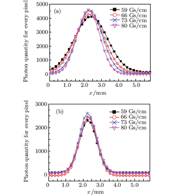 | Fig. 8. Fitting curves of horizontal one-dimensional profiles of the absorption images along the atom cloud center at different magnetic field gradients, obtained by (a) the closed-channel method and (b) the open-channel method. |
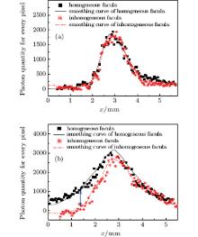
In order to discuss the influence of the inhomogeneity of the probe light field, an attenuator is used to weaken the left light field in the cross section of the probe laser and to produce inhomogeneous facula. For the open-channel method, the left wing of the inhomogeneous facula curve is symmetric compared with the right wing of the curve and the curves of inhomogeneous and homogeneous faculae are roughly the same, which can be seen in Fig. 9(a). The results of the closed-channel method are shown in Fig. 9(b). Compared with the homogeneous facula situation, the left part of the atom cloud absorbs fewer photons in the inhomogeneous facula situation; therefore, the curve is lower than the homogeneous facula curve on the left wing while the right wing is roughly the same as that of the homogeneous facula curve. Obviously, the curve is not symmetric for the inhomogeneous facula situation, which demonstrates that the closed-channel method cannot avoid the influence of the inhomogeneity of light field. The inhomogeneity of the light field may be regarded as the inhomogeneity of the atom distribution, which may lead to the detection inaccuracy.
 | Fig. 9. Horizontal one-dimensional profiles of the absorption images along the atom cloud center in the homogeneous facula situation and in the inhomogeneous facula situation, respectively, obtained by (a) the open-channel method and (b) the closed-channel method. |
Two absorption imaging methods are investigated to detect the quantity and distribution of a cold atom cloud. Theoretically and experimentally, the open-channel method proves to be superior to the closed-channel method. Because of the difference in the transition principles, the open-channel method absorbs fewer photons and the absorption process ends quickly, this can avoid the influence of pulse duration, light intensity, magnetic field strength, and the inhomogeneity of light field. For the closed-channel method, the absorption process lasts in the whole pulse duration and many more photons are absorbed, therefore the detection results are strongly affected by the above parameters. In general, the open-channel method is more reliable to image the cold atoms in magnetic field region and can be used in many areas, such as monitoring the evolution process of an atom cloud and measuring the temperature of the cold atoms.
The authors thank Mr. Wang Tong-Yu in Michigan State University and Associate Prof. Ding Ming in Beihang University for our in-depth discussions.
| 1 |
|
| 2 |
|
| 3 |
|
| 4 |
|
| 5 |
|
| 6 |
|
| 7 |
|
| 8 |
|
| 9 |
|
| 10 | [Cited within:2] |
| 11 | [Cited within:2] |
| 12 |
|
| 13 |
|
| 14 |
|
| 15 |
|
| 16 |
|
| 17 |
|
| 18 | [Cited within:1] |
| 19 |
|
| 20 |
|
| 21 |
|