Estimation of spatially distributed processes using mobile sensor networks with missing measurements*
[Jiang Zheng-Xiana), b), c)†  , Cui Bao-Tong
a), b) ]
, Cui Bao-Tong
 |


Corresponding author. E-mail: zhengxian@jiangnan.edu.cn
Project supported by the National Natural Science Foundation of China (Grant Nos. 61174021, 61473136, and 61104155) and the 111 Project (Grant No. B12018).
This paper investigates the estimation problem for a spatially distributed process described by a partial differential equation with missing measurements. The randomly missing measurements are introduced in order to better reflect the reality in the sensor network. To improve the estimation performance for the spatially distributed process, a network of sensors which are allowed to move within the spatial domain is used. We aim to design an estimator which is used to approximate the distributed process and the mobile trajectories for sensors such that, for all possible missing measurements, the estimation error system is globally asymptotically stable in the mean square sense. By constructing Lyapunov functionals and using inequality analysis, the guidance scheme of every sensor and the convergence of the estimation error system are obtained. Finally, a numerical example is given to verify the effectiveness of the proposed estimator utilizing the proposed guidance scheme for sensors.
Sensor networks have gained intensive research interest because of the very broad range of applications, encompassing gathering data, information processing, and surveillance.[1, 2] Filtering or state estimation is one of the most prime information processing problems in the sensor network and it has attracted the attention of many researchers.[3– 7] For example, Olfati-Saber et al.[8] presented a continuous Kalman consensus filtering algorithm on a mobile sensor network to tract two types of targets with stochastic linear and nonlinear dynamics. Wang et al.[9, 10] investigated the H∞ filtering problem for discrete-time nonlinear systems with or without time delay on a fixed sensor network.
In the majority of cases mentioned above, the target systems to be estimated were the finite dimensional systems described by ordinary differential equations. On the other hand, a wide class of processes are spatially distributed processes whose states evolve along both time and space and are described by partial differential equations (PDEs) which are commonly called the distributed parameter systems (DPSs) in the actual systems, such as chemical/radiation leaks, releasing toxic gas/fog, wildfire, oil spills, etc. The estimation of distributed parameter systems or their parameters has been investigated by many authors.[11– 15] A successful estimation of DPSs relies on not only the estimation algorithm but also on good measurements. This means that the redeployment of sensors in the fixed sensor network or the moving trajectory of mobile sensors which are used to measure the system states is a necessity to be considered. The related works that examine similar aspects of the mobile sensors in estimation of distributed parameter systems have appeared in Refs. [11], [14], and [16].
In reality there are various reasons that may cause missing measurements in sensor networks(such as measurement failure, intermittent sensor failures, or some collected data may be lost, etc.). The estimation problem with missing measurements has received much attention in recent years.[9, 10, 17] However, most systems that are to be estimated with missing measurements are described by ordinary differential equations. In almost all existing works, missing measurements have seldom been taken into account in the estimation of distributed parameter systems by using a mobile sensor network.
Therefore, the main purpose of this paper is to deal with the estimation for spatially distributed processes by using a mobile sensor network with missing measurements.
In this paper, we address the estimation for a spatially distributed process with missing measurements. Using Lyapunov stability arguments, the estimation error system is proved to be globally asymptotically stable in the mean square sense and a simple guidance law for every mobile sensor is given to improve the estimation performance for the spatially distributed process.
The problem formulation under consideration is described and the estimator of the spatially distributed process with missing measurements is given in Section 2, which is accomplished with the detailed discussion. In Section 3, we present the guidance policy for every mobile sensor and prove that the estimation error system is globally asymptotically stable in the mean square sense on the condition of missing measurements by using the Lyapunov stability theory. In Section 4, we give a case to verify the effects and advantages of our results. Finally, our conclusions are drawn in Section 5.
The target plant is a spatially distributed process whose state is to be estimated
where w(t, x) ∈ ℝ is the system state, along with the Dirichlet boundary value conditions w(t, 0) = w(t, l) = 0. t ∈ [0, + ∞ ) and x ∈ Ω = [0, l] denote the time variable and spatial variable, respectively. a(x) > a0 > 0 represents the diffusing coefficient.
The measurement outputs measured by sensors on the spatially distributed system are given by
where c(x; θ i(t)) denotes the spatial distribution of the i-th sensing device and yi is the measurement output by the i-th sensor. θ i(t) denotes the time-varying position of the i-th mobile sensor with the first-order dynamics governed by
where vi(t) is the velocity of the i-th mobile sensor. The stochastic variables ri(t) ∈ ℝ , i = 1, 2, … , n are Bernoulli distributed white noise sequences which are referred to the following distributed laws

where 

It is also assumed that the stochastic variables ri(t), i = 1, 2, … , n are mutually independent. Hence, the stochastic variables 

Remark 1 In this article the random variables ri(t), i = 1, 2, … , n in the measurement mode (2) are utilized to represent missing measurements or uncertain observations. The missing measurements were first put forward by Nahi, [18] and they were then widely used by many researchers.[9, 10, 19, 20]
In order to simplify stability analysis, it is assumed that the sensor network is an homogeneous network which consists of n identical sensing devices, and the spatial distribution of the i-th sensor which is onboard the i-th mobile agent is given by
or it can be written by c(x; θ i(t)) = H(θ i(t)− ε )− H(θ i(t)+ ε ), where H(θ i(t)− ε ) and H(θ i(t)+ ε ) are two Heaviside step functions.
Remark 2 The above assumption means that every sensing device is identical to each other in shape, and different only at the location θ i(t). The case of ri(t) = 1 means that the i-th sensor can provide the spatially averaged value of the state in the sense that
Another case of ri(t) = 0, which does happen in practice, implies that the measurements by the i-th sensor are missing.
One purpose of our work is to design a state estimator to approximate the state of the spatially distributed system (1) on the condition that there are missing measurements in the mobile sensor network (2). Another purpose is to design the motion velocity vi(t) of the i-th mobile sensor in order to yield a more efficient state estimator.
In order to employ Lyapunov methods for the stability analysis of the proposed estimation scheme and the guidance law of every mobile sensor, the above spatially distributed system (1) will be viewed in an abstract framework. Let 𝓦 be a Hilbert space which is equipped with the inner product 〈 · , · 〉 and induced norm | · | . Let 𝓥 be a reflexive Banach space with norm denoted by ∥ · ∥ , and assume that 𝓥 is embedded densely and continuously in 𝓦 .[11] Let 𝓥 * denote the conjugate dual of 𝓥 with induced norm ∥ · ∥ * . It follows that 𝓥 ↪ 𝓦 ↪ 𝓥 * with both embedding dense and continuously, and consequently we have | ϕ | ≤ c∥ ϕ ∥ , ϕ ∈ 𝓥 for some positive constant c.[11]
In this paper, 𝓦 = L2(Ω ) is the state space, where w(t, · ) = {w(t, x), 0 ≤ x ≤ l} denotes the state of spatially distributed system (1). The Sobolev space 𝓥 is given by 

where Dom(𝒜 ) = {ψ ∈ L2(Ω ) | ψ , ψ ′ abs. continuous, ψ ′ ′ ∈ L2(Ω ) and ψ (0) = ψ (l) = 0}. The operator 𝒜 is bounded and − 𝒜 is coercive, [11] in the sense that
The spatially distributed process (1) can then be rewritten as

The n output measurement operators are parameterized by the sensor locations θ i(t), i = 1, 2, … , n and they are given by

and the operator 𝓒 is given via

The output equation (2) can be rewritten as

where Γ (t) = diag(r1(t), r2(t), … , rn(t)), ri(t) is the stochastic variable.
Prior to giving the state estimator, we assume that the linear system (10) with the output measurement (11) is exponentially detectable.[21]
Here, we construct the following estimator, which makes use of the mobile sensor network with missing measurements to track the state w(t, x) of the target (1):
where ŵ (t) is the estimation of the system state w(t), K = diag(k1, k2, … , kn) > 0 is a used-defined n × n diagonal observer gain matrix and 
By setting e(t) = w(t) − ŵ (t), the evolution of the estimation error system can be obtained from Eqs. (10)– (12) as follows:
Let

then we have
Remark 3 Similar to the proof of Ref. [11], the coercivity and boundedness of the time-varying operator − 𝒜 c(θ (t)) can easily be proven. Indeed,
and
Moreover, 
The estimator error system (13) contains the stochastic quantity, so the notion of stochastic stability in the mean square sense for the estimator error system should be introduced.
Definition 1[20] The estimator error system (13) is said to be globally asymptotically stable in the mean square sense if the corresponding solution of system (13) satisfies

Remark 4 When the dynamic target model is described by an ordinary differential equation, the stochastic stability in the mean square sense for the estimator error system is discussed in Refs. [9] and [20]. Here, the dynamic target which is to be estimated is described by a partial differential equation (PDE). In the next section, we will discuss the stochastic stability in the mean square sense for the estimator error system (13).
Stability will be examined because the estimation error system and the guidance policies of the mobile sensors will be derived by using the Lyapunov stability arguments in the following theorem.
Theorem 1 Consider the mobile sensor network which is used to measure the state of the spatially distributed process (1) by the measurement mode (2) with missing measurements and the dynamic equations of sensors are governed by Eq. (3), where
Then, the proposed estimator (12) with the Lyapunov-based sensor guidance (18) is globally asymptotically stable in the mean square sense. The guidance policies for sensors enhance the estimator performance in the sense that the estimation error e(t) converges to zero faster than it would with the fixed sensor network.
Proof Choose the parameter-dependent Lyapunov functional candidate V(t) as follows:
where p is a positive constant, the operators 𝒜 and 𝒜 c are given by Eqs. (8) and (14), respectively. The coercivity of the operator − 𝒜 and − 𝒜 c follows from Eqs. (9), (17), so we have V(t) > 0.
The operator 𝓛 is defined as

then, along with the trajectory of the error system (15), we obtain

We consider the second term of Eq. (20). By using the fact 2〈 x, y 〉 ≤ 〈 x, x〉 + 〈 y, y 〉 , we have
Note that
and the stochastic variables 
After examining the third term of Eq. (20) carefully, we get
Based on Eqs. (20)– (23), we get
Because of the coercivity of the operator – 𝒜 in Eq. (9), the operator – 𝒜 c in Eq. (17) and the embedding, the following inequality holds

where d1 > 0 and d2 > 0 are the functions of the coercivity constant ν in Eq. (9) and the embedding constant c, respectively.[11] The choice of the positive constant 
From expression (26), we have

Since V(t) ≥ 0 and V(0) < ∞ , one can get 

Remark 5 In our work, the estimation for the spatially distributed process (1) is considered by using a mobile sensor network with missing measurements (2). As a special case, when ri(t) ≡ 1, t ∈ ℝ + , i = 1, 2, … , n, which means that there are no probabilistic missing data probabilities, as has been discussed by Demetriou in Ref. [11]. Compared to the idea measurement output, the estimation problem for the distributed parameter system with missing measurements is more practical.
Remark 6 In Theorem 1, the operator 𝒜 c(θ (t)) in Eq. (14) that depends on the parameter θ (t) is time-varying due to the spatial distribution 𝓒 i(θ i(t)) of the i-th mobile sensor. Based on the parameter-dependent Lyapunov function (19), we not have only proven that the proposed estimator (12) is globally asymptotically stable in the mean square sense but we have also given the motion velocity vi(t) of the i-th mobile sensor in Eq. (18) to enhance the estimator performance.
Remark 7 It should be noted that the velocity vi(t) of the i-th mobile sensor depends on the difference e(t, θ i(t) − ε ) − e(t, θ i(t)+ ε ) of the estimator error and 𝓒 i(θ i(t))e(t), which can be approximated by ε (e(t, θ i(t) − ε )+ e(t, θ i(t)+ ε )). The difference may be considered as the approximation of the spatial gradient of the error at the position θ i(t). When the spatial distribution in Eq. (6) is given by c(x, θ i(t)) = δ (x − θ i(t)), the above difference becomes the spatial gradient and the corresponding velocity vi(t) becomes

So the sensors that follow this scheme will be guided to the spatial regions of the highest gradient, which signifies the largest deviation of the error from its equilibrium.
Remark 8 Assume that every sensor is fixed, which means that 


The estimator is given by
then the estimator error e(t) = w(t)− ŵ (t) satisfies the following equation

In a similar fashion to the proof of Theorem 1, it is easy to get the following corollary.
Corollary 1 Consider the fixed sensor network which is used to measure the state of the spatially distributed process (1) by the measurement mode (27) with missing measurements. The proposed estimator (28) is then globally asymptotically stable in the mean square sense.
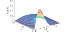
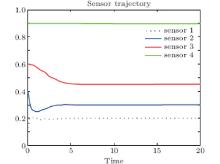
To demonstrate the proposed estimator (12) for the spatially distributed process (1), we consider the spatially distributed process (1) with the coefficient a(x) = 0.006, the initial condition set to w(0, x) = sin(π x)e− 10x2, x ∈ [0, 1] and for the estimator set to ŵ (0, x) = 0, x ∈ [0, 1]. For simplicity, the estimation error system (13) was simulated for 20 seconds with four mobile sensor agents whose initial positions were chosen as θ 1(0) = 0.1, θ 2(0) = 0.4, θ 3(0) = 0.6, θ 4(0) = 0.9. The positions for the four fixed sensors were chosen as 0.1, 0.4, 0.6, and 0.9. The spatial support ε = 0.04 was used for each sensor.
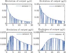
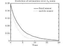
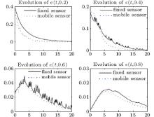
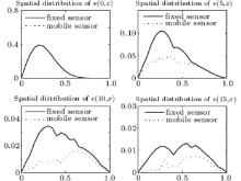
Figure 1 depicts the spatially distributed process (1) whose state evolves along both time and space. Figure 2 depicts the measurement outputs of the four mobile sensors with missing measurements. The evolution of the estimation error norm for both four fixed sensors and four mobile sensors with missing measurements is depicted in Fig. 3. It is observed that the norm of the estimation error e(t, x) for the mobile sensors converges to zero faster than that for the fixed sensors. Figure 4 depicts the estimation error system on the condition of missing measurements at four different positions. It is evident that the state error at different positions converges to zero by the mobile sensors or fixed sensors, and converges to zero much faster when the sensors are allowed to move. The estimation error system at four time instances is depicted in Fig. 5. Finally, the trajectory for the four mobile sensors is depicted in Fig. 6.
 | Fig. 1. The state of system (1). |
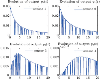 | Fig. 2. The outputs of the four mobile sensors with missing measurements. |
 | Fig. 3. The L2 norm of estimation error e(t, x). |
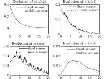 | Fig. 4. Estimation error versus time variable at different positions. |
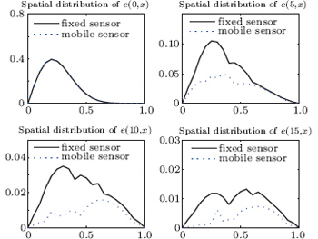 | Fig. 5. Estimation error versus spatial variable at different time instances. |
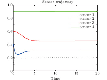 | Fig. 6. Sensor trajectories. |
The estimation problem has been discussed in this paper for the spatially distributed process by using a mobile sensor network with missing measurements. Both the estimator for the spatially distributed process and the guidance law for each mobile sensor have been presented by using Lyapunov stability arguments, which guarantee the estimation error system to be globally asymptotically stable in the mean square sense for all possible missing measurements. Finally, the simulation studies have revealed that a mobile sensor network could better enhance the estimation performance on the process state with missing measurements.
| 1 |
|
| 2 |
|
| 3 |
|
| 4 |
|
| 5 |
|
| 6 |
|
| 7 |
|
| 8 |
|
| 9 |
|
| 10 |
|
| 11 |
|
| 12 |
|
| 13 |
|
| 14 |
|
| 15 |
|
| 16 |
|
| 17 |
|
| 18 |
|
| 19 |
|
| 20 |
|
| 21 |
|
| 22 |
|
| 23 |
|
| 24 |
|