
Antagonistic formation motion of cooperative agents*
[Lu Wan-Ting, Dai Ming-Xiang, Xue Fang-Zheng† ]
]
]
|
|


Corresponding author. E-mail: xuefangzheng@cqu.edu.cn
Project supported by the National Natural Science Foundation of China (Grant Nos. 61203080 and 61473051) and the Natural Science Foundation of Chongqing City (Grant No. CSTC 2011BB0081).
This paper investigates a new formation motion problem of a class of first-order multi-agent systems with antagonistic interactions. A distributed formation control algorithm is proposed for each agent to realize the antagonistic formation motion. A sufficient condition is derived to ensure that all of the agents make an antagonistic formation motion in a distributed manner. It is shown that all of the agents can be spontaneously divided into several groups and that agents in the same group collaborate while agents in different groups compete. Finally, a numerical simulation is included to demonstrate our theoretical results.
Recent years have witnessed a considerable interest in the study of formation motion problems for multi-agent systems. In nature, formation motion widely exists in both the macrocosm and the microcosm, ranging from the movement of celestial bodies to electron motion, and from animal’ s flocking or schooling behavior to biological cell movement. Inspired by these natural phenomena, researchers have developed some important methods to realize the formation of a group of agents, such as robots, unmanned airborne vehicles (UAVs), and so on.
In many situations the formation motion problem can be regarded as a kind of consensus problem. Numerous studies have been conducted on formation motion problems.[1– 15] For example, article[16, 17] shows that animal formation motion requires the individuals to stay together so as to avoid predators or forage feed. As a matter of fact, in many cases, some agents achieve and maintain a desired formation by cooperating with others; however, some agents might collaborate while others oppose. As in Ref. [18], a bipartite consensus control algorithm for every agent to reach their own consensus as well as form two adversary group is proposed. Although there are many results on the formation motion for agents with an allied relationship, [19– 27] only a few results are obtained on formation motion for agents with allied/adversary relationships. When white blood cells go after invaders, they besiege the invaders rapidly through allied/adversary formation once they find the invaders’ position. Inspired by such biological formation motion, in this paper a new formation motion problem is first proposed for multi-agents with antagonistic interactions. On the one hand, each agent achieves a several-group antagonistic formation and each group is opposed with another. On the other hand, agents in allied groups collaborate with each other.
The outline of this paper is as follows. In Section 2, we define the consensus problems of formation motion on graphs. In Section 3, we present the relevant model and discuss the problem under investigation. The formation control algorithm is designed for each agent and the stability of the close-loop multi-agent system is analyzed in Section 4. Section 5 presents one numerical example to illustrate the formation control algorithm. Finally, our concluding remarks are stated.
The following notation will be used throughout this paper. ℝ m and ℂ m represent the set of all m-dimensional real and complex column vectors; ⊗ denotes the Kronecker product; 1 represents [1, 1, … , 1]T with compatible dimensions (sometimes, we use 1n to denote 1 with dimension n); 0 denotes zero value or zero matrix with appropriate dimensions.
Let 𝒢 (𝒱 , ℰ , 𝒜 ) be a signed graph of order n, where 𝒱 = {s1, … , sn} is the set of nodes, ℰ ⊆ 𝒱 × 𝒱 is the set of edges, and 𝒜 = [aij] is a weighted adjacency matrix. The node indexes belong to a finite index set ℐ = {1, 2, … , n}. An edge of 𝒢 is denoted by eij = (si, sj). The element aij of 𝒜 is nonzero if and only if the edge (si, sj) ∈ ℰ , whose head is i and tail is j in the directed graph 𝒢 while the order is irrelevant for undirected graphs. For the signed graph 𝒢 , there exists a sign mapping σ : ℰ → {+ , – } such that the edge set ℰ = ℰ + ∪ ℰ – . ℰ + = {(i, j)| aij > 0} and ℰ – = {(i, j)| aij < 0} are the sets of positive and negative edges, respectively.
The adjacency matrix 𝒜 is defined as aii = 0. The set of neighbors of node si is denoted by Ni = {sj ∈ 𝒱 : (si, sj) ∈ ℰ }. The out-degree of node si is defined as 
Lemma 1[28] If the undirected graph 𝒢 is connected, then the Laplacian L of 𝒢 has the following properties: (i) Zero is one eigenvalue of L, and 1 is the corresponding eigenvector, i.e., L1 = 0. (ii) The other n-1 eigenvalues are all positive and real.
How to achieve the antagonistic formation motion of cooperative multi-agents has important theoretical and practical significance, but it is also a big challenge to us at present. This paper attempts to investigate this complicated problem. For convenience of description, we take the four-group antagonistic formation motion of cooperate multi-agents into consideration here.
Consider a multi-agent system consisting of n agents. Each agent is regarded as a node in an undirected graph 𝒢 . Each edge (si, sj) ∈ ℰ corresponds to an available information channel between agents si and sj. Suppose that the i-th agent si (i ∈ ℐ ) has the following dynamics:

where the vectors xi ∈ ℝ m denote the state of the agent si and ui ∈ ℂ m is the control input.
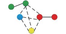
The n agents belong to four hostile groups 𝒱 1, 𝒱 2, 𝒱 3, and 𝒱 4, where 𝒱 = 𝒱 1⋃ 𝒱 2⋃ 𝒱 3⋃ 𝒱 4. Agents are opposite in different groups while they are cooperative in the same group. Thus, the interaction network of a multi-agent system can be described by a signed graph 𝒢 = (𝒱 , ℰ , 𝒜 ). For example, in Fig. 1, the solid and dashed edges, respectively, denote the allied and opposed relationships between agents. For convenience we use the positive and negative weights to describe such relationships from signed graph theory. In this model, the agents are required to move in four opposite directions surrounded by a target location to form the antagonistic formation.
 | Fig. 1. The antagonistic interaction network. |
In the formation control problem, a target formation vector di ∈ ℝ m is assigned to each agent i ∈ 𝒱 from the beginning. Here, we define each target formation vector having the same value; that is, the center of the antagonistic formation. All agents have to move to the target location by collecting information from its neighbors. We say that the antagonistic formation is achieved for the multi-agent system if the states of all agents satisfy

for some positive constant ς .
In this paper, our objective is to propose a distributed formation control algorithm using local and neighbor information to enable multi-agent systems to move into four antagonistic groups, where each group is convergent.
In this section, we study four-group antagonistic formation problems of the multi-agent system (1). The control algorithm is given by

for any i ∈ ℐ .
In control algorithm (3), the sgn(· ) is a sign function. The term Aq = diag{b1, b2} has four different forms, and each form represents one kind of relationship (antagonistic or cooperate). Between the agent of group 1 and the agent of group 2 we have b1 = – 1, b2 = 1, and let Aq = A2. Similarly, between the agent of group 1 and the agent of group 3 we have b1 = – 1, b2 = – 1, and let Aq = A3. Between the agent of group 1 and the agent of group 4 we have b1 = 1, b2 = – 1, and let Aq = A4. Apparently, if the agent belongs to one of the specific group, that is to say, there is a cooperation relationship between two agents, we have b1 = 1, b2 = 1, and let Aq = A1.
Denote x(t) = col(x1, … , xn) ∈ ℝ m× n, and d = col(d1, … , dn) ∈ ℝ m× n. With the control algorithm (3), the network dynamics can be written as
where L* can be seen as a special Laplacian and consists of five parts correspondingly, and L0⊗ Im is the matrix of the diagonal elements of L* specially. The others, L1, L2, L3, L4 are the Laplacians of the graph 𝒢 in four different conditions. L1 is also the matrix corresponding to the situations aij > 0 and Aq = A1. L2 corresponding to aij < 0 and Aq = A2. L3 corresponding to aij < 0 and Aq = A3. L4 corresponding to aij < 0 and Aq = A4.
Theorem 1 Consider a network of first-order agents with fixed topology that is kept connected. Four-group antagonistic formation can be achieved with the given control algorithm (3).
Proof Donate D = diag{σ 1, σ 2, σ 3, σ 4, … , σ n}, where σ 1 = diag{– 1, – 1}, σ 2 = diag{1, – 1}, σ 3 = diag{1, 1}, σ 4 = diag{– 1, 1}, they present four antagonistic groups, if there exists a cooperation relationship between two agents, then σ n is the same as that group. For example, if agent n and agent 1 are in the same group, then σ n = σ 1 = diag{– 1, – 1}. Then we have another transformation:

where z = x– d and ξ = [ξ 1, ξ 2, … , ξ 2n]. With this transformation, let Lσ = DL* D satisfy the condition of the Laplacian of a weighted undirected graph. The system can be rewritten as

According to Lemma 1, we can easily obtain that zero is one eigenvalue of Lσ and 1 is the corresponding eigenvector, i.e., Lσ 1 = 0. The other n– 1 eigenvalues are all positive and real.
Let ξ = β 1+ ε , where β = Ave(x(0)) is an invariant quantity and ε ∈ ℝ n satisfies Σ iε (i) = 0. We refer to ε as the disagreement vector. The vector ε is orthogonal to 1 and belongs to an (n– 1)-dimensional subspace, which is called the disagreement eigenspace of Lσ , provided that 𝒢 is strongly connected. Moreover, ε evolves according to the disagreement dynamics given by

The solution of the system (6) globally asymptotically converges to Ave(x(0)) (average-consensus is reached). Then the positive-define and proper Lyapunov function is given as follows:

Due to the fact that 1Tu = – (1TLσ )ξ ≡ 0. Thus, β = Ave(x(0)) is an invariant quantity. This allows the decomposition of ξ in the form of ξ = β 1+ ε . Therefore, we calculate 

This guarantees that V is a valid common Lyapunov function for the disagreement system (7). Moreover, we have

Then, we get

Furthermore, the disagreement vector ε vanishes exponentially quickly with the least rate of

Then, by Lyapunov theory, we have

Thus, the multi-agent system (1) with the control algorithm (3) reaches a consensus of four-group antagonistic formation.
Remark 1 From Eq. (13) we know ε (t) = 0, so ξ = β 1+ ε (t) = β 1 where β = Ave(x(0)). Also from Eq. (5), it means that | ξ 1| = | ξ 2| = · · · = | ξ 2n| = Ave(x(0)); that is, the position absolute value of each agent is the same to the average value. It is the Aq that decides the sign of position value, thus all of the agents reach a consensus of four-group antagonistic formation.
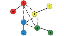
In this section, a numerical simulation is given to show the theoretical results obtained in the previous sections. The graph 𝒢 in Fig. 2 is the communication topology for the multi-agent system (1).
 | Fig. 2. The communication topology for the multi-agent system (1). |
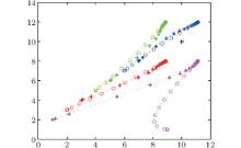
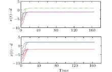
Example 1 Consider a multi-agent system with the interaction network illustrated in Fig. 2. The agents 1, 5 and agents 2, 6 and agents 3, 7 and agents 4, 8, respectively, belong to four adversary groups. For simplicity, it is assumed that the weight of each edge is 1 or – 1 based on their relationship. Figure 3 shows the trajectories of all agents with the control algorithm (3), the black cross denotes the target position. The trajectory lines of different colors, respectively, represent four antagonistic groups of the agents’ motion trail. The agents spontaneously move into four-group antagonistic formation from different initial position with the control algorithm (3). Furthermore, figure 4 shows the final position of the four-group antagonistic formation of the multi-agents. It is obvious that all of the agents finally reach a consensus of four-group antagonistic formation. It is shown that the cooperated multi-agents superpose each other well. Suppose that the target position of the eight agents is (10, 10), according to Theorem 1, the final antagonistic errors are, respectively, given by col(1.125, 2), col(– 1.125, 2), col(– 1.125, – 2), and col(1.125, – 2) for agents i ∈ {1, 5}, i ∈ {2, 6}, i ∈ {3, 7}, and i ∈ {4, 8}, which are validated by Fig. 5. Moreover, Figure 5 shows the tracking errors of eight agents and these errors are exactly what we used to form the four-group antagonistic formation.
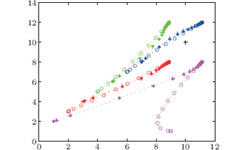 | Fig. 3. Trajectories of the multi-agent system (1). |
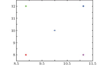 | Fig. 4. Final antagonistic formation of the multi-agent system (1). |
 | Fig. 5. The evolutions of tracking errors ei(t) = xi(t)– di ∈ ℝ 2 for i = 1, … , 8. |
In this paper, we have studied a new antagonistic formation motion problem for cooperative multi-agent systems. Firstly, with the help of signed graph theory we formulate the problem. Then, a formation control algorithm has been proposed for all agents to move into four antagonistic groups. Under the proposed control algorithm, proof has been presented to ensure the effectiveness of the four-group antagonistic formation control. Finally, a numerical simulation is included to demonstrate our theoretical results. This paper mainly investigates a four-group antagonistic formation motion and obtained the corresponding results. In a similar way, it is possible to expand this result to more antagonistic groups.
| 1 |
|
| 2 |
|
| 3 |
|
| 4 |
|
| 5 |
|
| 6 |
|
| 7 |
|
| 8 |
|
| 9 |
|
| 10 |
|
| 11 |
|
| 12 |
|
| 13 |
|
| 14 |
|
| 15 |
|
| 16 |
|
| 17 |
|
| 18 |
|
| 19 |
|
| 20 |
|
| 21 |
|
| 22 |
|
| 23 |
|
| 24 |
|
| 25 |
|
| 26 |
|
| 27 |
|
| 28 |
|