Coupled oscillators have been intensively studied in various disciplines because they have a variety of applications, including pattern recognition, biological information processing, and control.^{[1– 7]} Very recently, the dynamics of special networks of coupled oscillators has received particular attention in the literature.^{[8– 11]} In Ref. [8], the authors investigated different dynamical states of synchronization in a ring of four mutually inertia coupled self-sustained electrical systems, which are described by coupled Rayleigh– Duffing equations, and presented the stability properties of periodic solutions and transition boundaries between different dynamical states using the Floquet theory. In Refs. [9] and [10], the dynamic behaviors and synchronization of a ring of mutually coupled van der Pol oscillators were studied. The dynamics of a ring of unidirectionally coupled autonomous Duffing oscillators was studied in Ref. [11]. Although the individual uncoupled system has only one globally stable equilibrium, the system transits into periodic, quasi-periodic, and chaotic behaviors with an increase in coupling strength.

In practice there are many oscillators which do not interact with each other continuously, such as the species-food model in biology, the information transfer and exchange in ants, and the model of an integrated circuit. Very recently, impulsively coupled oscillators that are assumed to interact with each other only at discrete times have drawn considerable attention.^{[12– 16]} Pulse coupled neural networks which are special impulsively coupled oscillators have been utilized for various image processing applications, including image segmentation, feature generation, face extraction, motion detection, and so on.^{[12, 13]} In Ref. [14], a kind of impulsively coupled complex dynamical systems was introduced and several criteria related to the eigenvalues and eigenvectors of coupling matrix for synchronizing the impulsively coupled complex dynamical systems were established. In Ref. [15], a class of impulsively coupled complex switched networks with parametric uncertainties and time-varying delays was introduced and the robust synchronization of the presented model was studied. In Ref. [16], the authors introduced the concept of partial contraction theory of impulsive systems and investigated the synchronization problem of impulsively coupled oscillators. On the other hand, networked dynamical systems can achieve synchronization without interacting with each other continuously.^{[17– 20]} In Refs. [17]– [19], a kind of impulsive control protocol has been introduced for networked linear and nonlinear dynamical systems, respectively.

On the other hand, the dynamics of a system with an impulsive effect has attracted increasing attention.^{[21– 31]} In Ref. [21], the authors investigated the bifurcation and chaos observed in coupled Bonhoeffer– van der Pol (BVP) neurons with external impulsive forces. A class of periodic motions of an inverted pendulum forced by impulsive periodic excitation was analyzed in Ref. [22]. In Ref. [23], the authors investigated the effect of periodic forcing and impulsive perturbations on the predator– prey model with Holling type-II functional response. The onset of nontrivial periodic solutions for an integrated pest management model which is subject to pulsed biological and chemical controls was investigated in Ref. [24]. In Refs. [25]– [27], the dynamical behaviors of a linear impulsive system and a prey– predator system with impulsive control were discussed, respectively. In Ref. [28], the complex dynamics of the Chen system via an impulsive force was investigated and the Floquet theory was used to explore the non-smooth bifurcation mechanism for the periodic solutions. Furthermore, Floquet theory has been extended to explore the bifurcation mechanism for the periodic solutions of the Logistic map via periodic impulsive forces in Refs. [29] and [30].

In this paper, the complex dynamics of the non-smooth system which is unidirectionally impulsively coupled by three Duffing oscillators in a ring structure is studied both theoretically and numerically. The main contributions of this paper include: 1) the analytical expression of the Jacobian matrix of Poincaré map is derived by constructing a proper Poincaré map; 2) the two-parameter Hopf bifurcation sets are given by combining the shooting method and the Runge– Kutta method; and, 3) complex behaviors of the system are explored when the period is fixed and the coupling strength changes, and the stability of the periodic solutions of the system and their bifurcations are studied by using the Floquet theory.

The remainder of this paper is organized as follows. In Section 2, the system model is formulated. In Section 3, a bifurcation analysis of impulsively coupled Duffing oscillators is presented. In Section 4, bifurcation and chaos in impulsively coupled Duffing oscillators are explored when the impulsive coupling period is fixed and the impulsive coupling strength is considered as a bifurcation parameter. Finally, our conclusions are drawn in Section 5.

Notation Throughout this paper, the superscripts ‘ – 1’ and ‘ T’ stand for the inverse and transpose of a matrix, respectively; ℝ ⁿ denotes the n-dimensional Euclidean space; Let ℝ ₊ = [0, ∞ ), ℕ = {0, 1, 2, … }, ℤ ₊ = {1, 2, … }; ℝ ^{n× m} is the set of all n× m real matrices; For a vector x ∈ ℝ ⁿ, let | | x| | denote the Euclidean vector norm, i.e., ; j is the imaginary unit with the property j² = − 1.

Consider the autonomous Duffing oscillator described by the following second-order ordinary differential equation (ODE):

where a and d are positive constants. In this paper, the fixed parameters a = 0.1, d = 0.3 are used. Introducing the new coordinates x = v, y = v̇ to Eq. (1), the dynamics of the Duffing oscillator can be described as

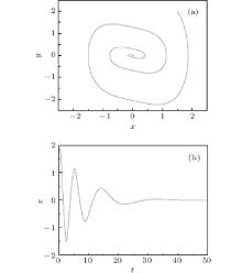
The system (2) only has one single stable equilibrium point at (x, y) = (0, 0), which is shown in Fig. 1.

Fig. 1.

	Figure Option ViewDownloadNew Window
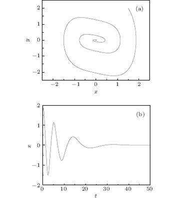	Fig. 1. Phase portrait and time histories of system (2) at a = 0.1 and d = 0.3.

Consider the ring of unidirectionally impulsively coupled Duffing oscillators, as shown in Fig. 2. The dynamics of impulsively coupled Duffing oscillators can be described by the following system

where τ is the impulsive coupling period, h is the impulsive coupling strength,

i = 1, 2, 3. Assume that xⁱ(t⁺ ) = xⁱ(t), yⁱ(t⁺ ) = yⁱ(t), that is the solution (x¹(t), y¹(t), x²(t), y²(t), x³(t), y³(t)) of the system is right-continuous at kτ .

Fig. 2.

	Figure Option ViewDownloadNew Window
	Fig. 2. Schematic representation of the ring network.

Since impulsively coupled systems are high-dimensional non-smooth systems, bifurcation analysis methods for continuous systems are not available. Therefore, the bifurcation analysis methods for non-smooth systems proposed in Refs. [21], [24], [32], and [33] are adopted in this paper to explore the bifurcation phenomenon of impulsively coupled Duffing oscillators.

The solution of Eq. (3) is described as

and

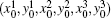
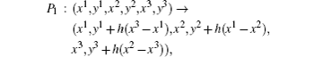
where is the initial value and i = 1, 2, 3.

Define the map P₁ as

and define the map P₂ as

Then, the Poincaré map P can be defined as P = P₂ ○ P₁, which is a composition of P₁ and P₂.

Let a fixed point of the Poincaré map P be u(x¹, y¹, x², y², x³, y³) and the fixed point satisfies

If the Poincaré map P has a fixed point, then the system has a periodic solution with period τ which is called a 1T-periodic solution. Similarly, if the Poincaré map P has a k-periodic point u(x¹, y¹, x², y², x³, y³), i.e., u = P^k(u) and u ≠ P^m(u), m = 1, 2, … , k − 1, then the system has a periodic solution with period kτ , which is called a kT-periodic solution.

The characteristic equation of the fixed point u of the Poincaré map P is

where DP(u) is the Jacobian matrix of the Poincaré map P at u.

The conditions for the bifurcations of the fixed point are given as follows:^[21]

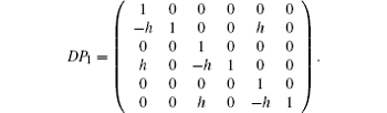
The Jacobian matrix of the Poincaré map P₁ is

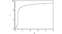
The numerical solution of the Jacobian matrix DP₂ of the Poincaré map P₂ can be determined by combining the shooting method and the Runge– Kutta method. Since P = P₂ ○ P₁, it follows that the analytical expression of the Jacobian matrix of Poincaré map is DP = DP₂ × DP₁. Now the impulsive coupling period and impulsive coupling strength are considered as bifurcation parameters, so that the bifurcation set and eigenvalues of the Jacobian matrix DP, i.e., the Floquet multipliers μ ₁, μ ₂, μ ₃, μ ₄, μ ₅, μ ₆ are obtained by solving Eqs. (5) and (6). Let h ∈ (0, 5], the Hopf bifurcation curve for the system is then obtained as depicted in Fig. 3. From Fig. 3, there exists a relation between the impulsive coupling period, impulsive coupling strength, and Hopf bifurcation. When the impulsive coupling period is larger, the impulsive coupling strength needs to be larger so that the system can generate a Hopf bifurcation. On the other hand, when the impulsive coupling period is smaller, the impulsive coupling strength needs to be smaller so that the system can generate a Hopf bifurcation.

Fig. 3.

	Figure Option ViewDownloadNew Window
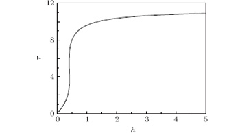	Fig. 3. Hopf bifurcation curve for system (3) at a = 0.1 and d = 0.3.

In this section, the impulsive coupling period is fixed at τ = 2 and the impulsive coupling strength h is considered as a bifurcation parameter. The effect of the parameter h on the system is considered by the stroboscopic map. The main idea is stated as follows: for a fixed h over a range, the numerical solution is first obtained; then, the stroboscopically sampling state of the system, i.e., the state of the system after periodic impulsive forcing, with period τ is obtained. Thus, the bifurcation diagram describing the effect of the impulsive forces can be attained. The stroboscopic map is a special case of the Poincaré map for periodically forced system or periodically pulsed system. Fixed points of the stroboscopic map correspond to 1T-periodic solutions of the system (3) whose period is τ ; periodic points of period k of the stroboscopic map correspond to kT-periodic solutions of the system (3) whose period is kτ ; invariant circles correspond to quasi-periodic solutions of the system (3).^[23]

The bifurcation and the Laypunov exponents diagrams of the system (3) are shown in Fig. 4. Here the Laypunov exponents of the system (3) are calculated by using the Poincaré map and the Gram– Schmidt orthonormalization method.^[32] From Fig. 4, when h > 0, as h increases, the system transits into stable, quasi-periodic, periodic, and hyper-chaotic solutions, etc. In the following, the dynamical behaviors will be analyzed by using the Floquet theory.

Fig. 4.

	Figure Option ViewDownloadNew Window
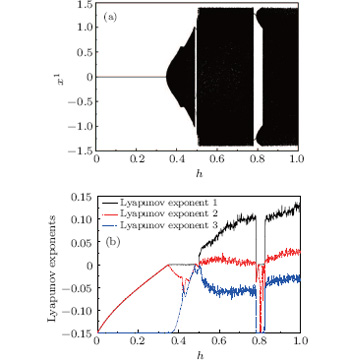	Fig. 4. Bifurcation and Laypunov exponents diagrams for system (3) under varying coupling strength h at a = 0.1 and d = 0.3.

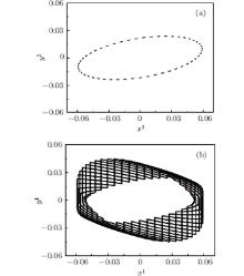
As can be seen from Fig. 4, when h < 0.349, the system shows a stable equilibrium solution and all of the Floquet multipliers lie inside the unit circle. At h = 0.349, a pair of two complex conjugate Floquet multipliers crosses the unit circle and the other Floquet multipliers stay inside the unit circle, so the Hopf bifurcation occurs and the equilibrium solution falls into a quasi-periodic solution, as shown in Fig. 5. This result is consistent with Figs. 3 and 4. Near h = 0.349, the Floquet characteristic multipliers are shown in Table 1.

Fig. 5.

	Figure Option ViewDownloadNew Window
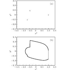
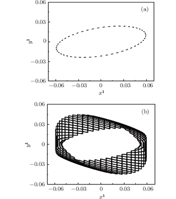	Fig. 5. Quasi-periodic solution for system (3) at a = 0.1, d = 0.3, and h = 0.35. (a) Stroboscopic map; (b) phase portrait.

Table 1.

Table 1.

Table 1. Floquet characteristic multipliers for system (3) at a = 0.1 and d = 0.3 (near h = 0.349). h μ 1, 2 | μ 1, 2| μ 3, 4 | μ 3, 4| μ 5, 6 | μ 5, 6| 0.309 0.3838 ± 0.8945i 0.9733 0.6289 ± 0.3915i 0.7408 0.2223 ± 0.5182i 0.5638 0.319 0.3722 ± 0.9065i 0.9800 0.6289 ± 0.3915i 0.7408 0.2127 ± 0.5180i 0.5600 0.329 0.3606 ± 0.9184i 0.9867 0.6289 ± 0.3915i 0.7408 0.2033 ± 0.5177i 0.5562 0.339 0.3488 ± 0.9301i 0.9934 0.6289 ± 0.3915i 0.7408 0.1940 ± 0.5173i 0.5525 0.349 0.3369 ± 0.9417i 1.0001 0.6289 ± 0.3915i 0.7408 0.1848 ± 0.5167i 0.5487

Table 1. Floquet characteristic multipliers for system (3) at a = 0.1 and d = 0.3 (near h = 0.349).

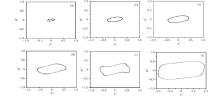
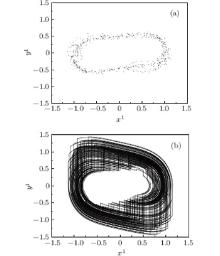
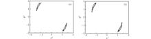
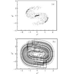
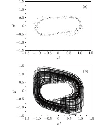
In Fig. 6, invariant circles are observed in the stroboscopic maps of the quasi-periodic solutions and these invariant circles gradually become large with their shape changing from smooth to non-smooth as h increases from 0.355 to 0.481. At h = 0.49888, the invariant circle loses its stability and the state moves to a stable 3T-periodic solution, as depicted in Fig. 7. Near h = 0.49888, a pair of two complex conjugate Floquet multipliers passes through the unit circle, one real Floquet multiplier jumps outside the unit circle and the other Floquet multiplier stays inside the unit circle. Hence, the 3T-periodic solution jumps to a chaotic solution instantly, which is shown in Fig. 8. Near h = 0.49888, the Floquet characteristic multipliers are shown in Table 2. At h = 0.5, the Laypunov exponents of the system are 0.02177, 0.00253, − 0.00629, − 0.04207, − 0.43896, and − 0.43951. Since there are two positive Laypunov exponents, the system is hyper-chaotic at h = 0.5.

Fig. 6.

	Figure Option ViewDownloadNew Window
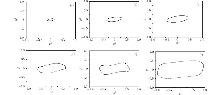	Fig. 6. Stroboscopic maps of quasi-periodic solutions for system (3) at a = 0.1 and d = 0.3. (a) h = 0.355; (b) h = 0.375; (c) h = 0.395; (d) h = 0.417; (e) h = 0.43; (f) h = 0.481.

Fig. 7.

	Figure Option ViewDownloadNew Window
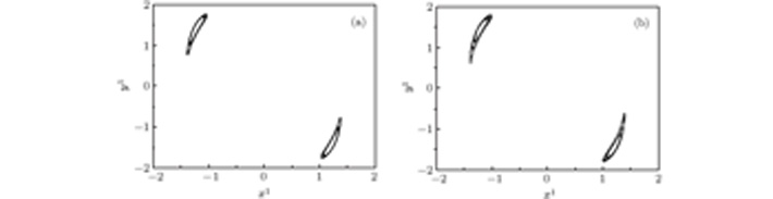
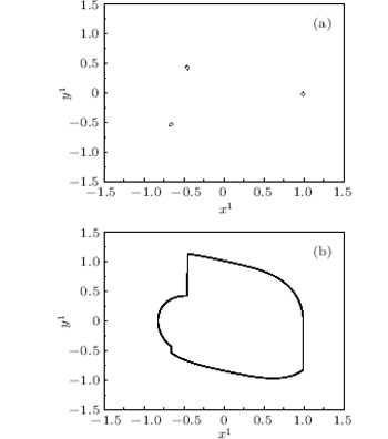	Fig. 7. 3T-periodic solution for system (3) at a = 0.1, d = 0.3, and h = 0.49. (a) Stroboscopic map; (b) phase portrait.

Fig. 8.

	Figure Option ViewDownloadNew Window
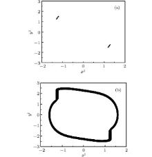
	Fig. 8. Hyper-chaotic attractor for system (3) at a = 0.1, d = 0.3, and h = 0.5. (a) Stroboscopic map; (b) phase portrait.

Table 2.

Table 2.

Table 2. Floquet characteristic multipliers for system (3) at a = 0.1 and d = 0.3 (near h = 0.49888). h μ 1, 2 | μ 1, 2| μ 3, 4 | μ 3, 4| μ 5, 6 | μ 5, 6| 0.49000 0.7403 ± 0.6531i 0.9872 0.8721 ± 0.1479i 0.8846 0.0465 ± 0.0612i 0.0768 0.49500 0.7967 ± 0.5733i 0.9815 0.8895 ± 0.1829i 0.9081 0.0471 ± 0.0587i 0.0753 0.49700 0.8403 ± 0.4908i 0.9731 0.9076 ± 0.2086i 0.9313 0.0476 ± 0.0567i 0.0740 0.49800 0.8745 ± 0.4089i 0.9654 0.9234 ± 0.2285i 0.9513 0.0480 ± 0.0551i 0.0731 0.49887 0.9421 ± 0.1076i 0.9483 0.9585 ± 0.2669i 0.9950 0.0485 ± 0.0521i 0.0711 0.49888 1.2836, 0.6829 1.2836, 0.6829 0.9837 ± 0.2897i 1.0255 0.0486 ± 0.0502i 0.0699

Table 2. Floquet characteristic multipliers for system (3) at a = 0.1 and d = 0.3 (near h = 0.49888).

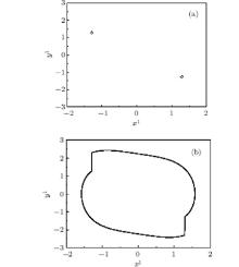
The hyper-chaotic attractor lasts until h = 0.779. At h = 0.779, there is a boundary crisis and the hyper-chaotic attractor suddenly jumps to a stable 2T-periodic solution, as depicted in Fig. 9. Thereafter, at h = 0.790, a pair of two complex conjugate Floquet multipliers crosses the unit circle and the other Floquet multipliers stay inside the unit circle. So another Hopf bifurcation occurs and the 2T-periodic solution becomes a quasi-periodic solution, which brings out two closed invariant circles, as shown in Fig. 10. Near h = 0.790, the Floquet characteristic multipliers are shown in Table 3. With the increase of the impulsive coupling strength, these two invariant circles become four invariant circles, eight invariant circles, and so on, which can be called a torus doubling bifurcation cascade.^[34] Finally, this torus doubling bifurcation cascade leads the quasi-periodic solutions to a chaotic solution, which is depicted in Figs. 11 and 12. At h = 0.825, the Laypunov exponents of the system are 0.09876, 0.00855, − 0.04798, − 0.20611, − 0.34228, and − 0.41643. Since there are two positive Lyapunov exponents, the system is hyper-chaotic at h = 0.825.

Fig. 9.

	Figure Option ViewDownloadNew Window
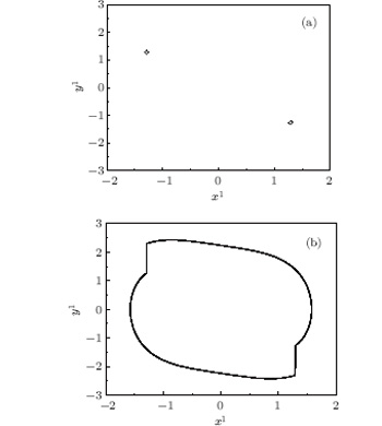	Fig. 9. 2T-periodic solution for system (3) at a = 0.1, d = 0.3, and h = 0.779. (a) Stroboscopic map; (b) phase portrait.

Fig. 10.

	Figure Option ViewDownloadNew Window
	Fig. 10. Quasi-periodic solution for system (3) at a = 0.1, d = 0.3, and h = 0.795. (a) Stroboscopic map; (b) phase portrait.

Table 3.

Table 3.

Table 3. Floquet characteristic multipliers for system (3) at a = 0.1 and d = 0.3 (near h = 0.790). h μ 1, 2 | μ 1, 2| μ 3, 4 | μ 3, 4| μ 5, 6 | μ 5, 6| 0.780 0.3199 ± 0.8232i 0.8832 – 0.5177 ± 0.1820i 0.5487 0.1232 ± 0.3172i 0.3402 0.784 0.2965 ± 0.8963i 0.9440 – 0.5172 ± 0.1834i 0.5487 0.1000 ± 0.3022i 0.3183 0.789 0.2669 ± 0.9622i 0.9986 – 0.5167 ± 0.1847i 0.5487 0.0804 ± 0.2900i 0.3010 0.790 0.2613 ± 0.9735i 1.0080 – 0.5167 ± 0.1848i 0.5487 0.0773 ± 0.2880i 0.2982

Table 3. Floquet characteristic multipliers for system (3) at a = 0.1 and d = 0.3 (near h = 0.790).

Fig. 11.

	Figure Option ViewDownloadNew Window
	Fig. 11. Stroboscopic maps for system (3) at a = 0.1 and d = 0.3. (a) h = 0.815; (b) h = 0.82.

Fig. 12.

	Figure Option ViewDownloadNew Window
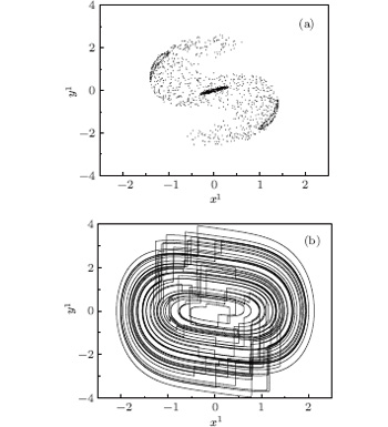	Fig. 12. Hyper-chaotic attractor for system (3) at a = 0.1, d = 0.3 and h = 0.825. (a) Stroboscopic map; (b) phase portrait.

This section only focuses on the dynamical behaviors of the system with the fixed period τ = 2. However, we can also obtain similar complex dynamical behaviors of the system with other periods and the proposed method can also be used to explore the bifurcation mechanism of these complex dynamical behaviors.

This paper has studied the complex dynamics of a non-smooth system which is unidirectionally impulsively coupled by three Duffing oscillators in a ring structure. The analytical expression of the Jacobian matrix of the Poincaré map has been derived by constructing a proper Poincaré map and the two-parameter Hopf bifurcation sets have been given by combining the shooting method and the Runge– Kutta method. In particular, the impulsive coupling period is fixed at τ = 2 and the impulsive coupling strength is considered as a control parameter. When the impulsive coupling strength h∈ (0, 0.349), the system has a stable equilibrium solution. At h = 0.349, the Hopf bifurcation of the stable equilibrium solution occurs and the system becomes a quasi-periodic solution. With a further increase of impulsive coupling strength from 0.349 to 0.490, the invariant circles change their shape and smoothness. At h = 0.490, the system suddenly jumps to a 3T-periodic solution and then to a hyper-chaotic solution thereafter. The hyper-chaotic solution lasts until h = 0.779, where it jumps to a 2T-periodic solution through a boundary crisis. Later on, the 2T-periodic solution becomes a quasi-periodic solution via a Hopf bifurcation at h = 0.790. This is followed by a torus doubling bifurcation cascade, which eventually leads to a hyper-chaotic solution. Numerical observations have shown that impulsively coupled oscillators can exhibit rich and complex dynamics. This research can improve the understanding and practical application of impulsively coupled nonlinear systems. Our future work will investigate the complex dynamics of large networks of impulsively coupled oscillators.