


Applications of modularized circuit designs in a new hyper-chaotic system circuit implementation*
[Wang Ruia) , Sun Huib)†  , Wang Jie-Zhi
c) , Wang Lud) , Wang Yan-Chaoe) ]
, Wang Jie-Zhi|
|


Corresponding author. E-mail: h-sun@cauc.edu.cn
Project supported by the Young Scientists Fund of the National Natural Science Foundation of China (Grant No. 61403395), the Natural Science Foundation of Tianjin, China (Grant No. 13JCYBJC39000), the Scientific Research Foundation for the Returned Overseas Chinese Scholars, State Education Ministry of China, the Fund from the Tianjin Key Laboratory of Civil Aircraft Airworthiness and Maintenance in Civil Aviation of China (Grant No. 104003020106), the National Basic Research Program of China (Grant No. 2014CB744904), and the Fund for the Scholars of Civil Aviation University of China (Grant No. 2012QD21x).
Modularized circuit designs for chaotic systems are introduced in this paper. Especially, a typical improved modularized design strategy is proposed and applied to a new hyper-chaotic system circuit implementation. In this paper, the detailed design procedures are described. Multisim simulations and physical experiments are conducted, and the simulation results are compared with Matlab simulation results for different system parameter pairs. These results are consistent with each other and they verify the existence of the hyper-chaotic attractor for this new hyper-chaotic system.
Chaotic systems have attracted increasing attention from different areas of science and engineering, such as encryption technology communication, control, chaotic economics, etc.[1– 5] Specifically, a chaotic oscillator has been used in encryption induced by sinusoidal signals.[6] This method can encrypt a message by using chaotic behavior, which it then transmits, thereby increasing the transmission security. Therefore, increasingly novel chaotic systems are generated from low-order chaotic systems to hyper-chaotic systems, and from two-wing systems to four-wing or multi-loop systems.[7– 9] With the deep development of chaotic systems, these systems are limited to not only the known parameter systems but also the parameter-estimating nonlinear chaotic system. A hybrid algorithm is implemented to solve the parameter estimation for chaotic systems.[10] Most chaotic systems are generated and verified by software, such as Matlab.[11] However, because of their future applications, such as usage in the confidential encryption communications, hardware simulation and physical verifications are also important for chaotic system generation. There are many different methods to realize physical hardware implementations for chaotic systems, such as basic circuit components like resisters, capacitors, DSP or FPGA technologies. Several different methods of implementing these circuits have been developed.[12– 16] For example, recently, in order to easily adjust chaotic systems with multiple parameters, a new hardware method has been developed for single-parameter adjustable chaotic systems.[17]
The modularized design method for chaotic circuits is a generalized circuit design method that is based on the state equations without dimensions for common chaotic circuit designs.[18– 23] There are two types of chaotic circuit modularized designs: one is the general modularized design, the other is the improved modularized design. The priority of the design procedure is to calculate the phase graph to determine the range of each variable. If the calculated range exceeds the practical circuit device dynamic range, then variable proportional compression is necessary. Otherwise, a differential– integral transformation will be used in the general modularized design, then the time scale transformation will be employed. However, an improved modularized design will omit the differential– integral transformation and use the time scale transformation directly. Correspondingly, this method will determine the device parameters by comparing state equations. This is the obvious difference between these two methods. That is, it is not necessary to transform differential equations into the integral form. Variable proportional unified compression transformation is easy to handle and to implement in the circuit. However, it may bring larger different values to the variables. Another compression transformation is heterogeneous. This provides different compression coefficient options, however, it is complex. Therefore, in this paper, we use unified compression transformation according to the characteristics of the system attractor. This improved method could determine the values of circuit components by directly making a comparison of the parameters of the state equations between before and after time scale transformation. Finally, hardware circuits will be implemented by using both methods. The accuracy of the simulation and experimental results generated by the improved modularized design is much higher than accuracy of the results obtained by the general method. In addition, less circuit parts are used.[12] However, the calculation of the circuit parameters is not intuitive.
The contribution of this paper is that an improved modularized design method is introduced into a new four-wing hyper-chaotic system circuit design. Specifically, an improved version of this method will be employed. The corresponding circuit implementation for this hyper-chaotic system is also proposed to show the accuracy and efficiency of the circuit implementation. The analog circuit implementation results match the Multisim and Matlab simulation results. Furthermore, this method can be applied to the implementation of other chaotic systems.
The rest of this paper is organized below. In Section 2 provides a specific application example for a new hyper-chaotic system, as well as detailed strategies and the procedure of calculations. Multisim simulations are also demonstrated in this section. In Section 3, the physical experimental results and comparisons among the Multisim, Matlab, and physical experiment results are presented. Finally, some conclusions are drawn from the present study in Section 4.
In this section a modularized design method will be implemented in a four-wing hyper-chaotic system. Multisim software is used to generate the circuit simulation results, and the corresponding physical circuit experiments are conducted to verify the hyper-chaotic attractor existence of this four-wing hyper-chaotic system.
Consider the four-wing autonomous chaotic dynamic system reported by Qi et al.[24]
This system has three state variables x, y, z, and five constant parameters a, b, c, d, and e.
When a = 14, b = 42, c = − 1, d = 16, and e = 4, there exists a typical four-wing chaotic attractor in system (1).
Wang[25] constructed a new four-variable system by varying the positive parameters a and b, fixing c = − 1, d = 16, e = 4, and then introducing a new state feedback controller w, which is shown below,

Wang[25] analyzed theoretically in detail the properties of this hyper-chaotic system and the Matlab simulation results for system (2), such as dissipativity, symmetry, equilibrium points, and so on. The dissipativity characteristics developed by Wang[25] are shown below

Therefore, the system (2) is dissipative when a+ b > 16. More characteristic descriptions can be found in Ref. [25] by Wang.
One typical Matlab simulation phase profile for the hyper-chaotic attractor of system (2) is shown in Fig. 1. A description of our Multisim and physical experiments using the improved modularized design method will be provided in detail in this paper. Figure 2 shows the flowchart of the improved modularized design for system (2). In this circuit design, several modules are used, such as an inverter module, an inverting summing module, and an inverting integrator module. To introduce the design method, we take a = 14 and b = 78 for system (2) as an example.
 | Fig. 1. Four-wing hyper-chaotic attractor x– y plane phase profile of system (2) with a = 14 and b = 78. |
 | Fig. 2. Hyper-chaotic system circuit design flowchart for system (2). |
Then system (2) becomes

First, we transform the time scales. Let τ = τ 0t, that is, transform the time scale of system (3). The bigger the value of τ 0, the faster the changing speed is and the denser the trajectory is, and vice versa. In general, τ 0 = 100. Then system (3) becomes

Second, we obtain the improved modularized circuit of system (2). This hyper-chaotic system circuit is composed of fundamental op-amp circuits, as shown in Fig. 3. Simultaneously, a corresponding x-channel circuit is also shown in Fig. 3, where variables x, y, z represent each state of the system and the channel output, respectively.
 | Fig. 3. Fundamental op-amp circuits used in system (4) circuit implementation, showing (a) inverting summing amplifier circuit, (b) inverting constant-gain multiplier circuit, (c) inverting integrator circuit, and (d) x-channel circuit. |
Third, we calculate the circuit component parameters R and C by using the modulus of the multiplier 0.1. Analogue amplifiers (LF347N) are used to implement the addition and integral operations. Multipliers (AD633JN) are used in output nonlinear terms.
Then, the system (4) is transformed into the following form according to Fig. 3:

Compare the parameters in system (5) with those in system (4) and list the corresponding equation group, then solve the parameters. Therefore, R1 = R2 = 72 kΩ , R3 = 25 kΩ , R4 = 1 MΩ , R5 = 62.5 kΩ , R6 = 100 kΩ , R7 = 1 MΩ , R8 = 13 kΩ , R9 = 100 kΩ , R10 = 100 kΩ , R11 = 667 kΩ are used in the Multisim circuit.
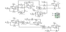
The Multisim simulation circuit of system (5) is shown in Fig. 4 with power voltage ± 15 V. Figure 4 shows the complete simulation circuit. In general, let R12 = R13 = R14 = R15 = R16 = R17 = 10 kΩ , C1 = C2 = C3 = C4 = 10 nF.
 | Fig. 4. Multisim simulation circuit for system (5). |
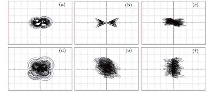
The corresponding attractor phases for different planes of system (5) are shown in Fig. 5.
 | Fig. 5. The attractor phase profiles for system (5) in (a) x– y plane, (b) x– z plane, (c) x– w plane, (d) y– z plane, (e) y– w plane, (f) z– w plane. The scale for each axis is 50 V/div. |
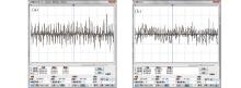
Comparing Fig. 5(a) with Fig. 1, the result generated from Multisim is close to that from Matlab. Since analog devices in Multisim are ideal, the variable outputs of the system might be very close to or exceed the voltage range of the practical amplifier linear region. However, it is hard to manipulate a practical device not to exceed the voltage limitation such as the characteristics shown in Fig. 6. Therefore, it is necessary to compress the variables. In general, it is guaranteed that the variable output voltage does not exceed ± 13.5 V.
 | Fig. 6. The variable responses for system (5) in (a) x– y plane with 100 V/div axis scale, and (b) z– w plane with 50 V/div axis scale. |
This design employs variables unified compression transformation; that is, the compression coefficients for each variable are equal.
Let the compression coefficients be k1, k2, k3, and k4, then

By substituting Eq. (6) into Eq. (3), we then have
Since this is the unified compression, the compression coefficients k1 = k2 = k3 = k4 = k, then
Compress Eq. (8) 20 times; that is, the compression coefficient for system (8) is k = 0.05. Then

Compare the parameters in Eq. (5) with the corresponding coefficients in Eq. (9), the resistances can then be calculated, and R1 = R2 = 72 kΩ , R3 = 1.25 kΩ , R4 = 1 MΩ , R5 = 62.5 kΩ , R6 = 5 kΩ , R7 = 1 MΩ , R8 = 13 kΩ , R9 = 5 kΩ , R10 = 100 kΩ , and R11 = 33 kΩ are employed in the Multisim circuit and experiments. Simultaneously, let R12 = R13 = R14 = R15 = R16 = R17 = 10 kΩ , C1 = C2 = C3 = C4 = 10
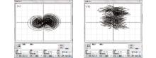
 | Fig. 7. Attractor phase profiles for system (3) after 20-time uniform compression in (a) x– y plane, (b) x– z plane, (c) x– w plane, (d) y– z plane, (e) y– w plane, and (f) z– w plane. Axis scales for planes x– y, x– z, x– w are all 5 V/div, axis scales for planes y– z, y– w, z– w are all 2 V/div. |
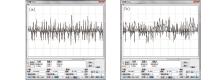
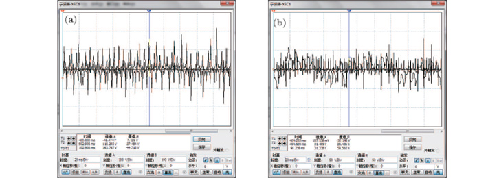
Correspondingly, figure 8 shows the variable responses after 20-time compression and indicates that the variable voltage outputs do not exceed the amplifier linear region.
 | Fig. 8. Variable responses after 20-time uniform compression for system (3) in (a) x– y plane with 5 V/div axis scale, and (b) z– w plane with 2 V/div axis scale. |
By comparing Figs. 7 and 8 with Figs. 5 and 6, it is shown that after compression the phase profiles have the same characteristics as before the compression and the output voltages do not exceed the amplifier linear region. In general, this is a better choice for the circuit experiment to guarantee that the outputs voltage does not exceed ± 13.5 V.
According to Fig. 4 and the chosen values of resistor and capacitor after compression, we set up the circuit. The voltage of the power supply for this design is ± 15 V. The voltage of the power supply for amplifier LF347N is in a range from ± 3.8 V to ± 18 V and the voltage of the power supply for multiplier AAD633JN is in a range from ± 8 V to ± 18 V. The attractor phase profiles in different planes are then recorded on a digital oscilloscope and the result is shown below.
By comparing Figs. 9(a), 7(a), and 1, it is can be seen that the phase profiles on oscilloscope for hardware circuit, Multisim simulation results, and Matlab simulation results are consistent with each other. Therefore, this four-wing hyper-chaotic attractor for system (2) is proven when a = 14 and b = 78 by the hardware circuit through the module method.
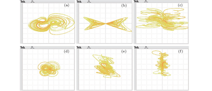 | Fig. 9. System (3) phase profiles for different planes after compression: (a) x– y plane, (b) x– z plane, (c) x– w plane, (d) y– z plane, (e) y– w plane, and (f) z– w plane. |
Other experiments for different choices of system parameters a and b are also conducted.
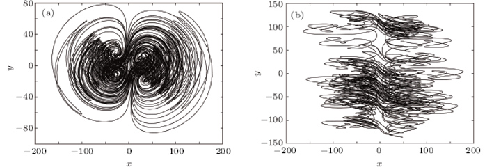
Case 1 When a = 4.38 and b = 43, some circuit resistor values can be calculated, and R1 = R2 = 228 kΩ , R3 = 25 kΩ , R4 = 1 MΩ , R5 = 62.5 kΩ , R6 = 100 kΩ , R7 = 1 MΩ , R8 = 23 kΩ , R9 = 100 kΩ , R10 = 100 kΩ , and R11 = 667 kΩ are used in Multisim simulation circuit. Let R12 = R13 = R14 = R15 = R16 = R17 = 10 kΩ , C1 = C2 = C3 = C4 = 10 nF. The Multisim simulation results are shown in Fig. 10. The corresponding Matlab simulation profiles are shown in Fig. 11. By comparing Figs. 10 and 11, it is shown that Multisim hardware simulation results are very consistent with the Matlab simulation results.
 | Fig. 10. Attractor phase profiles for system (2) when a = 4.38 and b = 43 in (a) x– y plane with channel A scale 50 V/div and channel B scale 20 V/div, (b) x– z plane with channel A scale 50 V/div and channel B scale 20 V/div, (c) y– w plane with channel A scale 20 V/div and channel B scale 50 V/div, and (d) x– w plane with channel A scale 50 V/div and channel B scale 50 V/div. |
 | Fig. 11. Four-wing hyper-chaotic system attractor phase graphs using Matlab when a = 4.38 and b = 43: in (a) x– y plane, (b) x– z plane, (c) y– w plane, (d) x– w plane. |
Case 2 When a = 14 and b = 43, some circuit resistor values can be calculated, and R1 = R2 = 72 kΩ , R3 = 25 kΩ , R4 = 1 MΩ , R5 = 62.5 kΩ , R6 = 100 kΩ , R7 = 1 MΩ , R8 = 23 kΩ , R9 = 100 kΩ , R10 = 100 kΩ , R11 = 667 kΩ are used in the Multisim simulation circuit. Let R12 = R13 = R14 = R15 = R16 = R17 = 10 kΩ , C1 = C2 = C3 = C4 = 10 nF. The Multisim simulation results are shown in Fig. 12. The corresponding Matlab simulation profiles are shown in Fig. 13. Comparing Fig. 12 with Fig. 13, it is obviously shown that Multisim hardware simulation results are well in accordance with the Matlab simulation results. However, the phase outputs obtained from Multisim exceed the amplifier linear region.
 | Fig. 12. Attractor phase graphs for system (2) when a = 14 and b = 43 in (a) x– y plane with channel A scale 50 V/div and channel B scale 50 V/div, and (b) x– w plane with channel A scale 50 V/div and channel B scale 50 V/div. |
 | Fig. 13. The four-wing hyper-chaotic system attractor phase profiles obtained by using Matlab in (a) x– y plane, and (b) x– w plane. |
Therefore, it is necessary to compress the coefficients uniformly to guarantee the accuracy of the phases in the physical circuit. Based on the analysis in Subsection 3.3, the coefficients of system (2) are compressed 10 times for these two cases. The components are then chosen by calculations and the results are shown below.
Case i When a = 4.38 and b = 43, then R1 = R2 = 228 kΩ , R3 = 2.5 kΩ , R4 = 1 MΩ , R5 = 62.5 kΩ , R6 = 10 kΩ , R7 = 1 MΩ , R8 = 23 kΩ , R9 = 10 kΩ , R10 = 100 kΩ , and R11 = 67 kΩ are used in experiments. Let R12 = R13 = R14 = R15 = R16 = R17 = 10 kΩ , C1 = C2 = C3 = C4 = 10 nF be used in experiments. A comparison of the phase profile for one plane between Multisim and physical experimental results after compression is made in Fig. 14.
 | Fig. 14. The phase profile for x– z plane obtained from Multisim after compression (a) (Channels A and B scales are 5 V/div and 2 V/div), and the phase profile obtained from digital oscilloscope (b) when a = 4.38 and b = 43 for system (2). |
Case ii When a = 14, b = 43, then R1 = R2 = 72 kΩ , R3 = 2.5 kΩ , R4 = 1 MΩ , R5 = 62.5 kΩ , R6 = 10 kΩ , R7 = 1 MΩ , R8 = 23 kΩ , R9 = 10 kΩ , R10 = 100 kΩ , and R11 = 67 kΩ are used in experiments. Let R12 = R13 = R14 = R15 = R16 = R17 = 10 kΩ , C1 = C2 = C3 = C4 = 10 nF. A comparison of the phase profile for one plane between Multisim and physical experiment results after compression is made and shown in Fig. 15.
 | Fig. 15. The phase profile for x– w plane obtained from Multisim after compression (a) (Channels A and B scales are both 5 V/div), and the phase graph obtained from oscilloscope (b), when a = 14 and b = 43 in system (2). |
From the above comparisons for different options of parameters a and b for system (2), physical realizations are obtained and the existence of the hyper-chaotic attractor is proved. Furthermore, it is also verified by the Multisim and Matlab simulation results. The improved modularized method provides a reliable straightforward method of realizing chaotic circuits. This method is easy to handle, and compression coefficients could avoid the output voltage being over the limitation of the amplifier linear region efficiency. The chaotic system implementation method can be widely used in many types of chaotic system circuit implementation, not only in hyper-chaotic systems but also in the scroll grid attractor chaotic system circuit implementation, and may also be used in encryption, secret communication, etc. Our future research will focus on the above-mentioned applications of this hyper-chaotic system.
In this paper, a hyper-chaotic system is electronically constructed by using an improved modularized circuit design method. Besides the introduction of the modularized design methods, the detailed design procedure is specifically proposed. In the meantime, a specific example for a new hyper-chaotic system is analyzed. Based on the design strategy, Multisim simulation circuits are built and the simulation results are verified. In addition, according to the characteristics of the practical circuit components, unified compression transformation is employed to determine the component values. Physical experiments for this hyper-chaotic system are implemented. Comparisons among Multisim simulation, Matlab simulation results, and physical experimental results show that they are consistent with each other and demonstrate that an attractor of the hyper-chaotic system exists. This method can also be used in other chaotic systems. In addition, the application of this hyper-chaotic system to encryption and secret communication will be considered and investigated by the method proposed in this paper in the near future.
| 1 |
|
| 2 |
|
| 3 |
|
| 4 |
|
| 5 |
|
| 6 |
|
| 7 |
|
| 8 |
|
| 9 |
|
| 10 |
|
| 11 |
|
| 12 |
|
| 13 |
|
| 14 |
|
| 15 |
|
| 16 |
|
| 17 |
|
| 18 |
|
| 19 |
|
| 20 |
|
| 21 |
|
| 22 |
|
| 23 |
|
| 24 |
|
| 25 |
|