


Self-adjusting entropy-stable scheme for compressible Euler equations*
[Cheng Xiao-Hana) , Nie Yu-Fenga)†  , Feng Jian-Hu
b) , Luo Xiao-Yuc) , Cai Lia) ]
, Feng Jian-Hu|
|


Corresponding author. E-mail: yfnie@nwpu.edu.cn
Project supported by the National Natural Science Foundation of China (Grant Nos. 11171043, 11101333, and 11471261) and the Doctorate Foundation of Northwestern Polytechnical University (Grant No. CX201426).
In this work, a self-adjusting entropy-stable scheme is proposed for solving compressible Euler equations. The entropy-stable scheme is constructed by combining the entropy conservative flux with a suitable diffusion operator. The entropy has to be preserved in smooth solutions and be dissipated at shocks. To achieve this, a switch function, which is based on entropy variables, is employed to make the numerical diffusion term be automatically added around discontinuities. The resulting scheme is still entropy-stable. A number of numerical experiments illustrating the robustness and accuracy of the scheme are presented. From these numerical results, we observe a remarkable gain in accuracy.
In this paper, we focus on constructing an entropy-stable scheme for solving compressible Euler equations. These equations are of great importance since they govern the dynamics of a compressible material, such as gases and liquids at high pressures, while neglecting viscous and heat fluxes. Mathematically speaking, Euler equations can be written as a system of nonlinear hyperbolic conservation laws. As we all know, shock waves, or contact discontinuities, may be contained in solutions of Euler equations due to their nonlinear hyperbolic nature. Once discontinuities are present, the theories of classical solutions are no longer meaningful. Hence, solutions are interpreted in a weak sense. Although weak solutions allow for discontinuities, they may not be unique in general. Thus, an extra entropy condition must be imposed to select the physically relevant solution.[1] Numerical schemes which are consistent with the entropy condition are later termed entropy-stable. For Euler equations, the entropy condition is a direct representation of the second law of thermodynamics. That is to say, the entropy, which is conserved in smooth solutions, should be dissipated at shocks. A numerical method which does not satisfy the entropy condition may lead to nonphysical solutions, such as negative densities and pressures. For example, the famous Roe scheme[2] violates the entropy condition at sonic points. Therefore, various entropy fixes[3, 4] have been proposed to modify the Roe scheme. These entropy fixes involve an artificial parameter that considerably depends on specific problems.
To achieve entropy stability, Tadmor introduced the concepts of entropy variable and entropy potential, and designed a class of entropy-conservative schemes, which are second-order accurate and conserve the entropy.[5, 6] A criterion was also provided for whether a scheme is entropy-stable or not, namely: three-point schemes are entropy-stable if they contain more viscosity than entropy-conservative schemes. Following this criterion, one can devise entropy-stable schemes by adding suitable diffusion operators to entropy-conservative schemes. This idea was applied to Euler equations by using the dissipative fluxes of physical viscosity and heat conduction.[7] However, the result is satisfactory only on very fine meshes. Moreover, the computation of entropy-conservative flux for systems of conservation laws is complicated and numerically expensive. To overcome this obstacle, Ismail and Roe presented a simple and computationally efficient entropy-conservative flux for Euler equations.[8] A methodology for constructing high order (than second) entropy-stable schemes was developed by Fjordholm et al. by combining high order entropy-conservative fluxes and suitable numerical diffusion operators involving an ENO reconstruction which satisfies the sign property.[9– 11]
In addition, other numerical schemes for Euler equations have been well-developed during the past few decades, such as the weighted essentially non-oscillatory (WENO) method, [12, 13] the discontinuous Galerkin (DG) method, [14, 15] the variational iteration method (VIM), [16– 18] and the meshless method.[19, 20] Among the variety of numerical methods, WENO and DG methods have been studied and enjoyed widespread popularity. Developed from the successful ENO scheme, [21] WENO schemes use the nonlinear weights to automatically achieve high order accuracy in smooth regions of the solution and an essentially non-oscillatory resolution at the discontinuities. Many WENO-type methods[22– 27] have been designed in recent years. The DG method was introduced by Reed and Hill[28] and further studied by Cockburn and Shu.[29– 33] To advance in time with high order Runge– Kutta methods, [34] the resulting schemes were termed RKDG schemes. Different limiters[35– 38] were constructed to suppress oscillations near shocks. However, to the best of our knowledge, rigorous stability results of these methods are still far from being complete, especially for nonlinear problems.
In the present article, we shall construct a self-adjusting entropy-stable scheme for compressible Euler equations. The new numerical flux contains two parts: entropy-conservative flux and a self-adjusting numerical diffusion term. The entropy-conservative part preserves the entropy exactly and performs well for smooth flows. However, it will give rise to oscillations in the vicinity of shocks. To eliminate such oscillations, a suitable numerical diffusion term is designed. Unlike the approach in Ref. [8], first order numerical diffusion is activated on the whole domain and makes the method less accurate in smooth regions. To avoid this, we utilize a switch function, which is based on entropy variables, to improve the accuracy of the entropy-stable method. The switch function’ s value possesses the property of being close to 1 at shocks and vanishing away from shocks so that the numerical diffusion works around discontinuities automatically. This is what we mean by ‘ self-adjusting’ . It should be noted that the introduction of the switch function does not affect the entropy stability.
The rest of the paper is organized as follows. In Section 2 we give a brief overview of Euler equations and the related entropy-stable theory. Section 3 describes the detailed procedure for designing the self-adjusting entropy-stable scheme for solving compressible Euler equations. A variety of test problems are presented in Section 4, with the aim of assessing how well the scheme performs in practice. Our conclusions are drawn in Section 5.
Without loss of generality, we consider the Euler equations for an ideal gas in two-dimensional (2D) space, written as a system of hyperbolic conservation laws,

where Ut = ∂ U/∂ t, F(U)x = ∂ F(U)/∂ x, and G(U)y = ∂ G(U)/∂ y, and the U, F, G vectors given by
Here, ρ is the density, p is the pressure, and (u, v) are the velocity components in x and y directions. The total energy is defined as

with the ideal gas constant γ = 1.4. This set of equations expresses the conservation laws for mass, momentum, and total energy. For simplicity, the spatial domain is discretized with a uniform mesh size (Δ x, Δ y). We denote the grid points by (xi, yj) with xi = iΔ x and yj = jΔ y. The domain is divided into cells Ii, j = [xi– 1/2, xi+ 1/2] × [yj– 1/2, yj+ 1/2] with midpoints xi+ 1/2 = (xi+ xi+ 1)/2 and yj+ 1/2 = (yj+ yj+ 1)/2. Then, a standard semi-discrete conservative finite difference (finite volume) scheme is given by
Here, Ui, j is the discrete solution at the grid point (xi, yj). Fi+ 1/2, j and Gi, j+ 1/2 are numerical fluxes consistent with F and G, respectively.
Assume that system (1) is equipped with a convex entropy function E = E(U), and associated entropy flux functions P = P(U) and Q = Q(U), such that the following compatibility conditions hold

For brevity of notions (• )′ is written for ∂ (• )/∂ U here. Then, it is straightforward to check that smooth solutions of Eq. (1) satisfy an additional conservation laws, also known as the entropy equality,

But for discontinuous solutions, the entropy has to be dissipated by implying the entropy inequality

(in a weak sense). Next, the formula (6) will be used as an essential component in our strategy to yield stable numerical schemes for Eq. (1) in this paper.
In this subsection, we describe the entropy-conservative scheme for 2D Euler equations. Here, entropy conservation means that the computed solutions satisfy the discrete entropy equality
with numerical entropy fluxes P ̃ i+ 1/2, j and Q ̃ i, j+ 1/2 consistent with P and Q. For convenience, let us introduce the following notation
Define the entropy variables as

and the entropy potentials as
Then, analogous to the one-dimensional (1D) case in Ref. [6], we give the two-dimensional entropy-conservative scheme by stating the following.
Proposition 1 The scheme (3) is entropy-conservative if the numerical fluxes F ̃ i+ 1/2, j and G ̃ i, j+ 1/2 satisfy the conditions
with numerical entropy fluxes

For Euler equations, the entropy pair is chosen to be

where s is the physical entropy given by s = ln p – γ lnρ . The above-defined entropy pair gives a simple form of entropy variables and entropy potentials
In general, the relations (11) provide two algebraic equations for several unknowns. Hence, the solutions of Eq. (11) are not unique. Although there are mainly three ways to compute entropy-conservative numerical fluxes for Euler equations, we will only describe Roe’ s explicit solutions here. Defining the parameter vectors z as
then the entropy-conservative fluxes in x and y directions are expressed by 

and
Here, 

An efficient computation of the logarithmic means is also given in Ref. [8]. We would like to mention that Roe’ s entropy-conservative numerical flux is not numerically expensive and is well-formed.
Entropy-conservative scheme preserves the entropy and performs well in smooth regions. However, it will produce oscillations near shocks. Thus, numerical diffusion operators should be added to ensure entropy stability. A scheme is said to be entropy-stable if the computed solutions satisfy the discrete entropy inequality
Define the following numerical fluxes,
where 

Proposition 2 The scheme (3) with numerical fluxes (20) is entropy-stable with the numerical entropy fluxes given by

Next, we will discuss the diffusion matrices in more detail. For simplicity, we will focus on the diffusion matrix 


Here, Ri+ 1/2, j is the averaged state of the right eigenvectors of ∂ F/∂ U,
Λ i+ 1/2, j is the diagonal matrix of absolute eigenvalues,

Si+ 1/2, j is a matrix of scaling factors,

such that R− 1 dU = SRT dV. All the averaged values in Ri+ 1/2, j, Λ i+ 1/2, j, and Si+ 1/2, j are determined exactly as in Ref. [8]. The remained Θ i+ 1/2, j, which is defined as

is a switch matrix that signals the amount of numerical diffusion to be added to the entropy-conservative scheme corresponding to each wave. We set 


and use the switch function proposed by Jamson[39]
The 

Remark 1 If one takes 
Remark 2 To generate ‘ enough’ entropy production across a shock, Ismail and Roe proposed to modify the eigenvalue matrix Λ i+ 1/2, j and the resulting fluxes were called entropy-consistent fluxes.[8]
In the following, a number of typical numerical examples are provided to illustrate the robustness and accuracy of the proposed scheme (ERoe-J). The results computed by the entropy-stable scheme (ERoe)[8] are also presented for a comparison. To complete the computation, a proper time discretization is needed. In the current work, we advance in time with the strong stability-preserving third-order Runge– Kutta (RK3) method, [40]

where
In all of the experiments below, the CFL number is taken as 0.3 and the time step is evaluated by

with the local sound speed 
Example 1 To test the accuracy of the proposed scheme, we consider the 1D Euler equations
with the initial data

and a 2-period boundary conditions. The exact solution is ρ (x, t) = 1 + 0.2 sin(π (x – t)), u(x, t) = 1, p(x, t) = 1. We compute the solution up to time t = 2. Table 1 presents the errors and convergence rates computed by ERoe and ERoe-J, respectively. It can be seen that ERoe-J gives errors of a smaller magnitude when compared with ERoe and achieves second-order accuracy in L1 norm. Thanks to the switch function the first-order numerical diffusion does not affect the overall accuracy of the scheme.
| Table 1. The errors and convergence rates of density ρ at t = 2. |
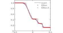
Example 2 Consider Sod’ s shock tube problem[41] with the initial data:

This initial continuity evolves into a left-going rarefaction wave, a right-going shock wave, and a right-going contact discontinuity. We compute the solution at time t = 0.16 on a mesh of 100 points. The obtained density is shown in Fig. 1. As one can clearly see, ERoe-J resolves all the waves better than ERoe.
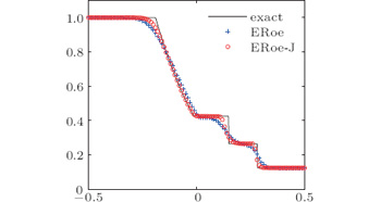 | Fig. 1. Density of Sod’ s shock tube problem. |
Example 3 Consider Toro’ s 123 problem[42] subject to the initial data:

The exact solution consists of two strong rarefaction waves and a trivial stationary contact discontinuity. Between the rarefactions, the pressure is very small (near vacuum) and this can lead to difficulties in numerical simulations. We compute the solution at time t = 0.1 on a mesh of 400 points. Figure 2 displays the results of density and internal energy. One can easily observe that ERoe-J produces a more accurate solution.
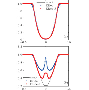 | Fig. 2. Solutions of Toro’ s 123 problem: (a) density and (b) internal energy. |
Example 4 We solve a long-time vortex advection problem[43] which describes the perturbations of a mean flow. The initial data are given by

with

Here, the temperature is defined as T = p/ρ and s is the physical entropy that was mentioned before. The initial center of the vortex is taken as (xc, yc) = (5, 5). The exact solution to this initial value problem is just the passive convection of the vortex with a velocity of 1 in x and y directions, i.e.

The computational domain is chosen to be [0, 10] × [0, 10] and we extend periodically in both directions. It is shown in Table 2 that ERoe-J achieves second-order accuracy in the 2D case. The computation is also performed on a mesh of 200 × 200 grid up to time t = 100. As one can see from Fig. 3, ERoe does not give a correct solution after long time simulation. To the contrary, ERoe-J preserves the vortex well.
| Table 2. The errors and convergence rates of density ρ at t = 10. |
 | Fig. 3. Solutions of the long-time vortex advection problem. Top: Plots of 30 density contour lines. Bottom: A density slice in x direction at y = 5 (numerical solution: circles, exact solution: line). |
Example 5 Consider the Riemann problems with initial data on [0, 1] × [0, 1] of the form
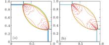
According to Ref. [44], there are 19 different admissible configurations separated by rarefaction (R), shock (S), and contact wave (J). We only show the results for the following two configurations.
Configuration 4 (Four shock waves)
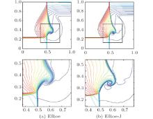
Configuration 19 (One shock wave, one rarefaction wave, and two contacts):

The computations are done on a 400× 400 grid and the density contour lines are shown in Figs. 4 and 5, respectively. Taking the results in Ref. [44] as reference solutions, we notice that ERoe-J achieves much better resolution than ERoe. For configuration 4, ERoe-J captures the shocks with less intermediate cells. And for configuration 19, ERoe-J resolves the wave structure more accurately (see the zoomed regions).
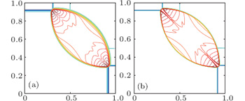 | Fig. 4. Configuration 4 with 30 density contour lines, t = 0.25: (a) ERoe, (b) ERoe-J. |
 | Fig. 5. Solutions of configuration 19 at t = 0.3. Top: Plots of 30 density contour lines. Bottom: Zoomed regions. |
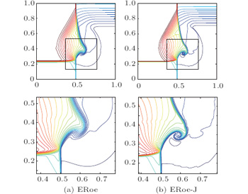
Example 6 We solve the double Mach reflection problem, originally from Ref. [45]. This is a standard test case for high resolution schemes. The computational domain is set to be [0, 4]× [0, 1] and the final time ist = 0.2. The reflecting wall lies along the bottom of the domain, beginning at x = 1/6. Initially, a right-moving Mach 10 shock, positioned at (x = 1/6, y = 0), makes a 60° angle with the reflecting wall and extends to the top of the domain. For the bottom boundary, the post-shock condition is imposed from x = 0 to x = 1/6 and a reflective condition is set from x = 1/6 to x = 4. At the top boundary, the values are set to describe the exact motion of a Mach-10 shock. The left and right boundaries are assigned to the inflow and outflow conditions, respectively. We consider a 480× 120 grid for this problem. The density contours of the solution are shown in Fig. 6. The WENO-LF-5 results[46] are provided as a reference solution. It is observed that ERoe produces a kinked Mach stem but ERoe-J avoids such a failure.
 | Fig. 6. Solutions of double Mach reflection problem. Left: Plots of 30 density contour lines. Right: Zoomed regions. |
In this paper, we have proposed a self-adjusting entropy-stable scheme to solve compressible Euler equations. Following Tadmor’ s idea, an entropy-stable scheme is designed by adding a suitable numerical diffusion to the entropy-conservative flux. To achieve self-adjustment, we introduce a switch matrix which signals the amount of numerical diffusion so that numerical diffusion is added to the entropy-conservative flux automatically. Our numerical experiments demonstrate a remarkable gain in accuracy of the proposed scheme.
| 1 |
|
| 2 |
|
| 3 |
|
| 4 |
|
| 5 |
|
| 6 |
|
| 7 |
|
| 8 |
|
| 9 |
|
| 10 |
|
| 11 |
|
| 12 |
|
| 13 |
|
| 14 |
|
| 15 |
|
| 16 |
|
| 17 |
|
| 18 |
|
| 19 |
|
| 20 |
|
| 21 |
|
| 22 |
|
| 23 |
|
| 24 |
|
| 25 |
|
| 26 |
|
| 27 |
|
| 28 |
|
| 29 |
|
| 30 |
|
| 31 |
|
| 32 |
|
| 33 |
|
| 34 |
|
| 35 |
|
| 36 |
|
| 37 |
|
| 38 |
|
| 39 |
|
| 40 |
|
| 41 |
|
| 42 |
|
| 43 |
|
| 44 |
|
| 45 |
|
| 46 |
|