When a fluid supports another heavier fluid in a gravity field or when a fluid accelerates another heavier fluid, the interface between the two fluids will be instable. The interfacial instability known as Rayleigh– Taylor instability (RTI)^{[1, 2]} was investigated firstly by Rayleigh and then Taylor. Subsequently, a number of works^{[3– 11]} have theoretically studied the RTI, especially on a planar interface in the Cartesian geometry. A small perturbation, η (x, t = 0) = ε cos(kx), grows exponentially in time initially, namely, η (x, t) ≈ η _Lcos(kx) with the linear amplitude η _L = ε e^{γ t}, where the linear growth rate is the Atwood number, ρ _l (ρ _h) is the density of the lighter (heavier) fluid, g is the acceleration, k = 2π /λ is the perturbation wave number with λ being the wavelength, ε [kε ≪ 1] is the initial perturbation amplitude of the interface, and t represents time. After a sufficient growth of the perturbation, kη _L is no longer small (typically kη _L∼ 1), and the flow enters the nonlinear regime, where the “ bubbles” of the lighter fluid rise through the denser fluid, and the “ spikes” of the heavier fluid penetrate down through the lighter one. Regarding this nonlinear growth regime, potential models^{[6– 10]} predicted that the bubble (spike) tip tends to move with a constant velocity (acceleration). Before the strong nonlinear growth regime, one has a weak one (0.628≲ kη _L≲ 1).

In the weakly nonlinear growth regime, for an initial single-mode cosine interface perturbation within the framework of third-order perturbation theory, ^{[6, 12– 15]} the interface, up to the second order, can be expressed as

This expression shows that the interface function η (x, t) consists only of oscillatory terms. This means that the equilibrium interface (the initially unperturbed interface) keeps rest in the weakly nonlinear growth regime. Regarding the planar RTI, many studies^{[16– 19]} have been performed.

In many applications, the RTI occurs in non-Cartesian geometries. For example, RTI plays a significant role in astrophysics, ^{[20– 23]} and the inertial confinement fusion (ICF).^{[24– 30]} Such systems with spherical or cylindrical geometries can be geometrically divergent (explosive) or convergent (implosive).^[31] Numerical simulation^[32] and experiments^{[33, 34]} predicted RTI existing at the cylindrical or spherical interface in the nonlinear regime, and that the character of the interface evolution is not relevant to bubble or spike, but closely related to the inward or outward portion of the interface. What mainly leads to the evolution difference between the planar and cylindrical interfaces? The related theoretical studies even in the weakly nonlinear regime are not explored.

This paper aims to fill a gap in the present knowledge on the previous development of cylindrical RTI. The investigation on the two styles of cylindrical RTI concludes that the interface function consists of two parts: oscillation and non-oscillation terms. At the same wavelength and in the limit of larger radius, oscillation terms in cylindrical RTI reproduce the planar results and non-oscillation terms tend to zero. Again, an interesting thing is that non-oscillation term has the uniform form regardless of divergent or convergent configuration. As a result, the non-oscillation term, which contributes nothing to the planar RTI, is an essential character of the cylindrical RTI in the weakly nonlinear regime, and the zeroth-order velocity just governed by this non-oscillation term is investigated in this paper.

Two incompressible, irrotational, and inviscid fluids of density ρ _h for the heavy fluid and ρ _l for the light fluid in a Cartesian (cylindrical) geometry with coordinates x, y, and z (r, θ , and ξ ) are subject to a steady acceleration g^p (g^c). An interface separating the two fluids is located at y = 0 (r = r₀ ≫ ε ). There are two unstable RTI configurations according to different arrangements of the fluids and directions of the interface acceleration. When the fluid of the density ρ _h occupies the space y > 0 (r > r₀), the fluid of the density ρ _l does the remaining space, and g^p = – ge_y (g^c = – ge_r). The interface is prone to RTI if there are perturbations on the material interface. The other RTI is vice versa. The evolution interfaces are denoted as y = η ^p₁, y = η ^p₂ (r = r₀ + η ^c₁ and r = r₀ + η ^c₂).

2.1. Convergent configuration

The governing equations are

and

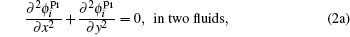
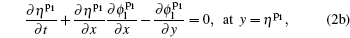
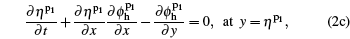
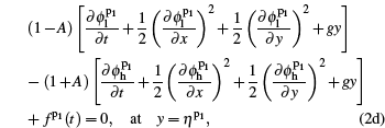
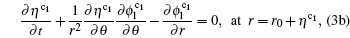
Here, superscripts p₁ and c₁ denote the Cartesian and cylindrical geometries, respectively, ϕ _i are velocity potentials for the two fluids with i denoting h or l, and f^p₁(t) (f^c₁(t)) is an arbitrary function of time. The Laplace equations Eq.(3a) and Eq. (4a) come from the incompressibility conditions. Equations (3b) and (3c), ((4b) and (4c)) represent the kinematic boundary conditions in Cartesian (cylindrical) geometry (i.e., the normal velocity continuous condition at the interface) that a fluid particle initially situated at the material interface remains at the interface afterwards. The Bernoulli equations (3d) and (4d) represent the dynamic boundary conditions, in which the pressure continues across the material interface.

Considering an initial perturbation η ^p₁(x, t = 0) = ε cos(k x) or η ^c₁(θ , t = 0) = r₀ + ε cos(nθ ), where the initial perturbation amplitude ε is much less than the initial perturbation wavelength λ (namely, ε ≪ λ ), and k and n are, respectively, the wave number and mode number. The interface displacement and the perturbation velocity potentials can be expanded into a power series in ε as

and

(5c)

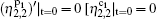
Note that the high harmonics are generated due to the nonlinear mode-coupling process, and the velocity potentials satisfy their Laplace equations. Additionally, amplitude coefficients s_{1, 1}(t), s_{2, 2}(t), and s_{2, 0}(t) with s denoting η , a, and b, where t will be omitted in the following expressions, are what we want to determine. Here, the initial velocities of the interface ∂ η ^p₁/ ∂ t|_t=0 = ∂ η ^c₁/ ∂ t|_t=0 = 0 are under our consideration.

Substituting Eqs.(4a)– (4c) ((5a)– (5c), in which O(ε ³) is ignored in the governing equations(2b)– (2d) ((3b)– (3d), and then expanding every term of these resulting equations in Taylor series at the unperturbed interface y = 0 (r = r₀), subsequently replacing η ^p₁ (η ^c₁) in the resulting equations with Eq.(4a) ((5a)) ignoring O(ε ³), we can obtain the first-order equations, just including terms of ε and the second-order equations consisting only of terms ε ². It is worth noting that the zeroth-order equations without ε determine nothing but f^p₁(t) (f^c₁(t)), which is unimportant for our concern.

2.1.1. First-order equations and solutions

As mentioned above, the first-order equations can be obtained as

and

where notation ' denotes the derivative with respect to time.

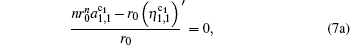
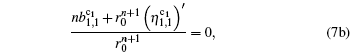
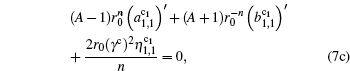
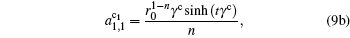
Expressing the variables and ( and ) from Eqs. (6a) and (6b) ((7a) and (7b)), respectively, and then substituting the expressions and ( and ) to Eq.(6c) ((7c)), we can obtain a second-order ordinary difference equation of η _{1, 1}. The corresponding initial conditions and are adopted, and the related solutions are

where is the planar linear growth rate, ^{[1, 2]} and

where is the cylindrical linear growth rate. This result is also predicted for uniform density incompressible limit by Yu and Livescu.^[31] In their work, ñ = A given by Eq.  (18) where ñ ² = n²/k_t| g| , n is the linear growth rate, is the mode number in the z direction and m is the one in θ . For the case in our paper, k_z = 0, and then k_t = m/r₀, leading to . Here, n and m, respectively, correspond to γ ^c and n in our paper.

2.1.2. Second-order equations and solutions

To solve the second-order equations, we need to separate terms, just including the second harmonic (the terms of cos(2kx) or cos(2nθ )) from the terms with the zeroth harmonic (without the term of cos(2kx) or cos(2nθ )), and then form the corresponding equations of the second harmonic and of the zeroth harmonic.

For the equations of the second harmonic, we have

and

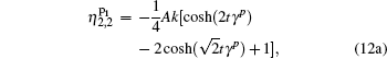
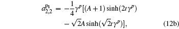
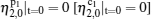
Note that the corresponding initial conditions are and , and . By the method mentioned above, the solutions of the second harmonic are

and

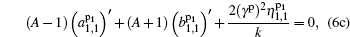
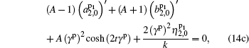
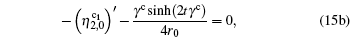
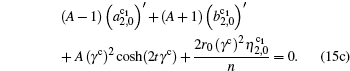
For the zeroth harmonic, we have

and

(15c)

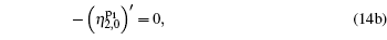
Note that equation (14a) ((15a)) is the same as Eq. (14b) ((15b)).

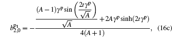
We first solve Eq. (14a) ((15a)) with the initial condition , then substitute this result into Eq.(14b) ((15b)) with A = – 1, subsequently solve and further work out . These results are

and

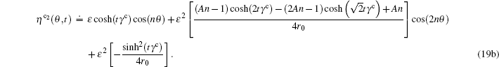
Therefore, the interface functions up to the second order are

2.2. Divergent configuration

The similar approach employed above can also be applied to this case by replacing A with – A and g with – g in Eqs. (2d) and (3d), and then replacing k with – k in Eqs. (4b) and (4c), and n with – n in Eqs. (5a)– (5c). Repeating the above procedure, we can obtain the analogy results. For simplicity, just interface functions up to the second order are, respectively, expressed as

Insight into the planar interface (19a) will be performed next. With time t, cosh(2tγ ^p) is much larger than , so that the latter term can be disregarded. From expression , we see that the term e^{– 2tγ p} contributes the stable effect to the interface. In the weakly nonlinear RTI, namely, after the linear stage of the RTI, the time t becomes large. These two aspects just mentioned are taken into account to determine the leading terms, so equation (19a) can be reduced to Eq. (1).

At the same initial perturbation wavelength λ , considering mode number n = 2π r₀/λ and wave number k = 2π /λ , we have n = kr₀ and then γ ^c = γ ^p. In addition, replacing n in Eq.(19b) with kr₀ and then taking the limit of r₀→ ∞ , we can reproduce the planar result (19a). These show that at the same wavelength, the cylindrical RTI has the same linear growth rate as planar RTI; and together with larger radius, the cylindrical evolution interface tends to the planar one.

Comparing the cylindrical result with the planar result, one sees that there exist two independent spatial scales in the cylindrical result, i.e., the radius r₀ and the wavelength λ , while only λ in the planar result.

It is worth noting that an interesting thing can also be found by comparing the interfaces in Cartesian and cylindrical domains. The non-oscillatory term – ε ²sinh²(tγ ^c) appearing in both cylindrical cases is an essential character different from the result of the Cartesian case. That is to say, whether for the convergent or divergent RTI, the non-oscillatory term keeps the same expression. Furthermore, this non-oscillatory term has nothing with θ . It is clear that this term is related to the initial unperturbed interface. What this non-oscillatory term contributes to the interface can be found by its derivative with respect to time (i.e., zeroth-order velocity v⁽⁰⁾) which is

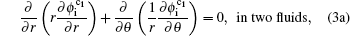
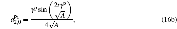
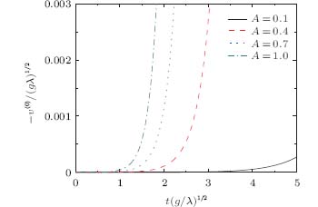
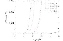
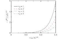
The evolutions of this velocity are shown in Figs. 1 and 2 where we use acceleration g and perturbation wavelength λ to normalize the velocity v⁽⁰⁾ and time t, and the initial perturbation amplitude is fixed as ε / λ = 0.001. Figure 1 shows the effect of Atwood number A on the v⁽⁰⁾. It is found that the magnitude of v⁽⁰⁾ increases with A, especially with A > 0.4. Figure 2 shows the effect of initial radius r₀ on v⁽⁰⁾. Note that as addressed above, the mode number n is proportional to radius r₀ at the same wavelength λ . Therefore, figure 2 also shows the effect of the mode number n on the v⁽⁰⁾. It is found that the magnitude of v⁽⁰⁾ decreases with r₀ (or n). As confirmed, v⁽⁰⁾ will tend to zero when r₀ → ∞ . In other words, the effect of the cylindrical geometry will vanish when r₀ → ∞ . Furthermore, the direction of v⁽⁰⁾ is inward (i.e., in the negative direction of axis r), which can be seen from Figs. 1 and 2, where the – v⁽⁰⁾/(gλ )^1/2 ≥ 0 is shown.

Fig. 1.

	Figure Option ViewDownloadNew Window
	Fig. 1. Normalized velocities – v(0)/(gλ )1/2 with normalized time t(g/λ )1/2 for different Atwood numbers: A = 0.1 (the solid line), A = 0.4 (the dashed line), A = 0.7 (the dotted line) and A = 1.0 (the dot-dashed line). The initial perturbation amplitude is fixed as ε / λ = 0.001.

Fig. 2.

	Figure Option ViewDownloadNew Window
	Fig. 2. Normalized velocities – v(0)/(gλ )1/2 with normalized time t(g/λ )1/2 for different initial radius r0/λ = 1 (the solid line), r0/λ = 2 (the dashed line), r0/λ = 3 (the dotted line), and r0/λ = 4 (the dot-dashed line). The initial perturbation amplitude is fixed as ε / λ = 0.001.

The Rayleigh– Taylor instability (RTI) at the interface separating two incompressible, irrotational, and inviscid fluids in the cylindrical geometry is explicitly investigated in this paper by the formal perturbation method up to the second order. There are two unstable RTI configurations according to different arrangements of the fluids and directions of the interface acceleration. These two styles of RTI: convergent and divergent configurations in cylindrical geometry compared with the planar RTI are taken into account. The uniform initial conditions including the same perturbation amplitudes and the rest interface are in our consideration. With the same initial perturbation wavelength λ , for the large initial radius of the cylindrical interface (i.e., r₀ → + ∞ ), the cylindrical interface can be reduced to the planar interface. Our explicit results lead to the following findings.

(i) There are two independent spacial scales (radius r₀ and wavelength λ ) in the cylindrical RTI; while there is only one spacial scale (λ ) in the planar RTI.

(ii) The cylindrical interface consists of two parts: oscillatory part similar to the planar result and non-oscillatory part which contributes nothing to the planar one. That is, the cylindrical interface velocity stems from the oscillatory and non-oscillatory terms. The velocity resulting from the non-oscillatory term is greatly concerned in this paper. It is found that the divergent configuration has the same zeroth-order velocity as the convergent one. This velocity increases with Atwood number A while decreases with the initial radius of the interface r₀ (or mode number n at the invariable wavelength λ ), and its direction is inward.