Rotating machinery such as steam turbine, compressor, fan, rolling mill, and machine tool is widely used in industrial production. The transmission system driven by an AC motor as a core part of rotating machinery plays an irreplaceable role in electricity, energy, transportation, metallurgy, and national defense fields. Torsional vibration in rotating machinery seriously influences the normal work and causes damage to the equipment. The mechanism and the control method for torsional vibration of rotating machinery were actively researched in recent years. For example, the nonlinear frequency response calculation of a torsional sub-system containing a clearance type nonlinearity was presented.^{[1, 2]} The studies showed that the nonlinear impact damping reduces the resonance peak and the area of quasi-periodic and chaotic motions. In Refs. [3] and [4], a nonlinear elastomeric damper or absorber was used to control the torsional vibrations of the crankshaft in internal combustion engines when subjected to both external and parametric excitation torques. Various nonlinear factors are contained in a rotating machinery system, which lead to the complex dynamic behaviors of the system, such as bifurcation and chaos.^{[5– 8]} These are the important reasons for the instability of the torsional vibration system. Abstracting the rolling mill main drive system into two masses or a multi-mass relative rotation system, the bifurcation and chaos of the torsional vibration of the system were studied.^{[9– 11]} A nonlinear feedback controller was also proposed to control the Hopf bifurcation point and the stability of the periodic solutions.

Time delay, as a kind of basic nature of the physical phenomenon, exists widely in industrial systems. It has a great influence on the analysis and the control of a system, such as leading to the instability of the system and the control law failure. However, reasonably introducing and processing the time delay can improve the performance of a system.^{[12– 14]} There has been extensive interest in studying the effect of the time delay on the dynamic system in different fields. Many important advances have been made in neural network systems, ^{[15– 17]} biological systems, ^[18] and control systems.^{[19– 21]} The time delay feedback control applied to suppress the vibration of the primary system was put forward by Olgac et al.^{[22, 23]} The critical feature of the technique is the utilization of a controlled time delay in the feedback loop, which is traditionally looked upon as an undesirable element in dynamic controls. A novel active vibration absorption device, the centrifugal delayed resonator, was presented as an efficient way of eliminating undesired torsional oscillations in rotating mechanical structures.^[24] It can eliminate the vibration of the primary system completely by adjusting the feedback and the time delay online. The effects of the time delay on dynamical behaviors such as stability, bifurcation, and chaos were investigated by introducing different forms of time delay feedback into a relative rotation system.^{[25, 26]} Zhao^{[27, 28]} found that with the method of time delay and nonlinear coupling, the vibration damping performance can be improved.

AC motors have been widely used in the transmission system of rotating machinery in recent years. The above papers better explained the mechanism and the control methods for torsional vibration of rotating machinery from the viewpoints of mechanical parameters. However, the effects of the electrical parameters were not taken into account. In this paper, a nonlinear electromechanical coupling model of the transmission system is established considering the coupling effect of the electrical and the mechanical parameters. By using a combination of analytical and numerical methods, the effects of the time delay on the stability and the Hopf bifurcation of the system are investigated rigorously. These provide a theoretical basis for design and control of the electromechanical coupling transmission system which is widely used in practical engineering.

The rest of this paper is organized as follows. Section 2 presents the dynamic equation of the electromechanical coupling transmission system and introduces a time delay feedback to control the dynamic behaviors of the system. Section 3 analyzes the stability of the linear time delay system based on the direct method. By choosing the time delay as a bifurcation parameter, Section 4 proves the existence of the Hopf bifurcation and also gives a formula for determining the direction of the Hopf bifurcation and the stability of the bifurcating periodic solutions. Numerical simulations are performed in Sections 3 and 5, and some concluding remarks are provided in Section 6.

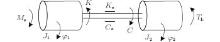
The rolling mill main drive system driven by an AC motor can be abstracted into a two-mass torsional vibration model, as shown in Fig. 1.

Fig. 1.

	Figure Option ViewDownloadNew Window
	Fig. 1. Dynamic model of the electromechanical coupling system driven by an AC motor.

The total kinetic and potential energies of the system can be described as

The dissipation function is

The air-gap magnetic field energy W_m between the stator and the rotor is

Here J_i (i = 1, 2) is the moment of inertia, φ (i= 1, 2) and φ _i (i = 1, 2) are the angle of rotation and the rotational speed, respectively, K is the torsional stiffness of the drive shaft, C is the shafting damping coefficient, C_e is the electromagnetic damping coefficient (generated by the rotor damper bar), R is the average radius of the rotor, and L_r is the effective length of the rotor.

The air-gap permeance per unit area between the stator and the rotor is

where Λ ₀ = μ ₀/σ , σ = k_μ δ ₀, μ ₀ is the air magnetic permeability, k_μ is the magnetic saturation, δ ₀ is the equivalent air-gap, x₃ and y₃ are the synthetic eccentrics, and α is the electric angle. For the geometrical dimensions of the air gap, we have

where x₀ and y₀ are the static eccentrics, ε ₂ is the dynamic eccentric, and x and y are the amplitudes of the transverse vibration. According to the electrical machine theory, the fundamental synthetic magneto motive force (mmf) between the stator and the rotor is

where F_sm and F_jm are three phase fundamental synthetic mmf amplitudes of the stator and the rotor, respectively. The phase angle of the rotor mmf lags behind the stator mmf ψ ₁ + ψ ₂ . Substituting the Lagrangian function L = T + W_m − V into the dissipation Lagrange equation

yields

where ∂ W_m/∂ φ ₁ is the electromagnetic torque, and T_L is the load torque. In the case of no eccentricity, , where

Define electromagnetic stiffness K_e as the coefficient of φ ₁, that is, K_e = k₁ . In order to control the dynamic behaviors of the electromechanical coupling system, the nonlinear time delay state feedback is introduced. Thus, the dynamic equation of the controlled nonlinear electromechanical coupling torsional vibration system becomes

Equation (11) is the nonlinear dynamic equation of the electromechanical coupling system with a time delay feedback, which is the basis of dynamic behavior analysis and control of the electromechanical coupling torsional vibration system. The effects of the time delay feedback on the stability and the Hopf bifurcation of the system are studied in the following sections.

Let .The equilibrium points of Eq. (11) can be transferred to the origin of the coordinates by a coordinate transformation. Thus studying the dynamic characteristics of the system equilibrium points at the origin is of universal significance. Considering the equilibrium points at the origin of the coordinates, we can reduce Eq. (11) to the first-order equation

where τ ₁, τ ₂ are time delays and β ₁, β ₂ are time delayed feedback gains. The characteristic equation of the linearized system (12) with time delay is

where .

The direct method^[23] is employed to analyze the system. Substitute e^{− τ ₁s}→ (1 − Ts)/(1 + Ts) (τ ₁ ∈ R⁺, T ∈ R) into Eq. (13) at s = ± iω _c. This is an exact substitution, which is different from the Taylor expansion and the Pade approach in essence. By the substitution, equation (13) becomes

The values of T are determined, where a change in the number of unstable roots takes place, according to the Routh– Hurwitz criterion. Then τ ₁ can be calculated by ω _c and T as

The above equation describes an asymmetric mapping in which one T is mapped into infinitely many τ ₁’ s for a given ω _c. Inversely for the same ω _c, one particular τ ₁ only corresponds to one T. The root tendency is

where n is the number of pure imaginary roots. The RT represents the direction of transition of the roots at iω _cn as τ ₁ increases from τ _1nl − ε to τ _1nl + ε . The RT = +1 represents that the root iω _cn crosses the imaginary axis from the stable left plane to the unstable right plane. There is a converse crossing direction of the roots when RT = − 1. So the number of unstable roots can be calculated by the following expressions:

where NU(0) is the number of unstable roots when τ ₁ = 0. Beginning from the smallest τ ₁, NU(τ ₁) increases by 2 if RT = +1 and NU (τ ₁) decreases by 2 if RT = − 1. We identify those regions in τ ₁ where NU(τ ₁) = 0 as stable and others as unstable.

The system parameters can be taken as , and l₂ = − 0.1. When β ₁ = 0.8, the values of T are T₁ = − 0.7965 and T₂ = − 0.4121. The root tendencies corresponding to them are RT = +1 and RT= − 1. The stable regions of the system are shown in Table 1. From the table, it can be seen that in the time delay regions (0, 3.4378), (4.4955, 8.0930), … , (30.8019, 31.3687), the system is stable and the length summation of stable regions, L, is 15.9309. With the increase of τ ₁, the characteristic roots move to the unstable right-half plane through the crossing point iω _c = ± 1.3497i, creating an increase in NU(τ ₁ ) by 2 each time. Thus the stable regions of the system can no longer be found. When β ₁ = 1, the values which imply the presence of one pair of imaginary roots are T₁ = − 1.0681 and T₂ = − 0.2688. The root tendencies are RT = + 1 and RT = − 1, respectively. The stable regions of the system are (0, 2.9811), (5.2910, 7.3429), and (11.1052, 11.7046), as shown in Table 2. The length summation of stable regions is 5.6323.

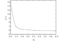
Tables 1 and 2 reveal that the stable regions of the system are different when the linear feedback gains are different. The relationship between L and β ₁ is analyzed when β ₁ increases from 0.8 to 4. As depicted in Fig. 2, the relationship between L and β ₁ is monotonously decreasing. As the linear feedback gain increases, the length summation of the stable regions drops. The appropriate feedback gain β ₁ will make the system stable for a given τ ₁.

Keeping the other parameters constant, the time history responses for different τ ₁ are shown in Fig. 3 when β ₁ = 1. Table 2 shows that τ ₁ = 2.5 and τ ₁ = 6 are all in the stable regions. It verifies the correctness of Table 2 that the time history responses gradually reduce to 0 in Figs. 3(a) and 3(b), and the convergence speed decreases with the increase of τ ₁. It can be seen from Table 2 that τ ₁ = 3.5 and τ ₁ = 8 are all in the unstable regions. The diverging time history responses in Figs. 3(c) and 3(d) are presented to confirm the prediction. The appropriate time delay τ ₁ will make the system stable for a given feedback gain β ₁.

Fig. 2.

	Figure Option ViewDownloadNew Window
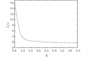	Fig. 2. The relationship between L and β 1.

Fig. 3.

	Figure Option ViewDownloadNew Window
	Fig. 3. Time history responses for different τ 1: (a) τ 1 = 2.5, (b) τ 1 = 6, (c) τ 1 = 3.5, (d) τ 1 = 8.

Table 1.

Table 1.

Table 1. The stable regions of τ 1 when β 1 = 0.8. τ 1 RT NU (τ 1) ω c(i) 0 3.4378 +1 1.3497 2 4.4955 – 1 1.1942 0 8.0930 +1 1.3497 ⋮ ⋮ ⋮ ⋮ 30.8019 – 1 1.1942 0 31.3687 +1 1.3479 2 36.0239 +1 1.3479 4 ⋮ ⋮ ⋮ ⋮

Table 1. The stable regions of τ 1 when β 1 = 0.8.

Table 2.

Table 2.

Table 2. The stable regions of τ 1 when β 1 = 1. τ 1 RT NU (τ 1) ω c(i) 0 2.9811 +1 1.4405 2 5.2910 – 1 1.0807 0 7.3429 +1 1.4405 2 11.1052 – 1 1.0807 0 11.7046 +1 1.4405 2 16.0664 +1 1.4405 4 ⋮ ⋮ ⋮ ⋮

Table 2. The stable regions of τ 1 when β 1 = 1.

The stable regions of the linear time delay electromechanical coupling system are obtained according to the above analysis. When τ ₁ crosses over the stable boundary, the system is in critical stable state and the Hopf bifurcation may occur. The limit cycles will generate near the equilibrium point when the Hopf bifurcation occurs and the nonlinear part of the system will affect the stability of the bifurcating periodic solutions.

4.1. Existence of the Hopf bifurcation

When τ ₁ = τ ₂ = τ , the dynamic equation of system (12) can be expressed as

where

and f(x_i, x_iτ ) is the nonlinear part. The associated characteristic equation of the linearized system (19) at the origin is

where .

When τ = 0, equation (20) becomes

where k₃ = p₃, k₂ = p₂ + m₂, k₁ = p₁ + m₁, and k₀ = p₀ + m₀. By the Routh– Hurwitz criterion, all roots of Eq. (21) have negative real parts if and only if

For τ ≠ 0, let λ = ω ₀ i and τ = τ ₀, and substitute these into Eq. (20). For the sake of simplicity, denote ω ₀, and τ ₀ by ω and τ , respectively. Separating the real and the imaginary parts, we obtain

By a simple calculation, equation (23) leads to

where q₃ . Since cos ²ω τ + sin ²ω τ = 1 , we have

where

By denoting z = ω ² , equation (26) becomes

Let . In order to investigate the dynamic behavior of bifurcation, we always suppose: (H₁) equation (27) has at least one positive real root; (H₂) Re[d λ (τ ₀)/(dτ )] ≠ 0.

Since , we conclude that if r₆ < 0, there exists a z₀ ∈ (0, + ∞ ) such that l(z₀)= 0.

Let z₀ be the smallest positive root of Eq. (27). Then is the positive root of Eq. (26). From Eq. (24) and the expression of Δ , we obtain

Taking the derivative of λ with respect to τ in Eq. (20), we obtain

Noticing Eq. (23), we have

where Δ > 0 and sign(Re[d λ (τ )/d τ ]|_{τ = τ 0}) = sign((Re[d λ (τ )/d τ ]|_{τ = τ 0})^{− 1}).

Now we can employ the result from Ruan and Wei^[29] to analyze Eq. (20), which is, for the convenience of the reader, stated as follows.

Lemma 1 Consider the exponential polynomial

where τ _i ≥ 0 (i = 1, 2, … , m) and P_j⁽ⁱ⁾ (j = 1, 2, … , n) are constants. As (τ ₁, τ ₂, … , τ _m) vary, the sum of the order of the zeros of P(λ , e^{− λ τ ₁}… , e^{− λ τ m}) on the right half plane can change only if a zero appears on or crosses the imaginary axis.

From Lemma 1, it is easy to obtain the following theorem.

Theorem 1 Suppose that (H₁), (H₂), and Eq. (22) hold, then the zero solution of system (19) is asymptotically stable for τ ∈ [0, τ ₀) and the system undergoes a Hopf bifurcation at the origin when τ = τ ₀.

4.2. Direction and stability of the Hopf bifurcation

In this section, the formulae for determining the direction of the Hopf bifurcation and the stability of the bifurcating periodic solutions of system (19) at τ ₀ will be presented by employing the normal form method and the center manifold theorem.^[30]

For convenience, let t = sτ , y_i(t) = x_i (τ t), and τ = τ ₀ + μ , μ ∈ R. Then system (19) is transformed into a functional differential equation in C = C([− 1, 0], R⁴) as

where , f: R × C → R⁴ are respectively given by

where . By the Riesz representation theorem, there exists a matrix function η (θ , μ ), (− 1 ⪁ θ ⪁ 0) whose components are bounded variation such that

In fact, choose

where δ is the Dirac delta function. For ϕ ∈ C[− 1, 0], define

Then system (31) is equivalent to

For ψ ∈ C¹ ([0, 1], (R⁴ * ), define

and a bilinear inner product

where η (θ ) = η (θ , 0). Then it is not difficult to show that A(0) and A^* are adjoint operators. From the discussion in Theorem 1, we know that iω ₀τ ₀ are eigenvalues of A(0). Therefore, they are also eigenvalues of A^*. Let be the eigenvector of A(0) corresponding to the eigenvalue iω ₀τ ₀. Thus, A(0)q(θ ) = iω ₀τ ₀q(θ ). From the definition of A (0), we have

Then by a direct computation, it is not difficult to show

Similarly, let be the eigenvector of A^* corresponding to − iω ₀τ ₀, and we can obtain

In order to assure ⟨ q^*(s), q(θ )⟩ = 1, we can choose M as

where is the conjugate imaginary of M.

Next we will compute the coordinate to describe the center manifold C₀ at μ = 0. Define

On the center manifold C₀, we have

where z and are the local coordinates for center manifold C₀ in the directions of q^* and . We are only concerned with the real solutions. For solution y_t ∈ C₀ of system (35), since μ = 0, we have

We rewrite this equation as

where

From Eqs. (37) and (38), we obtain

Substituting Eqs. (33) and (42) into Eq. (41), we have

where h.o.t. stands for higher order terms, and

Then we can obtain

Comparing the coefficients with Eqs. (41) and (43), we have g₂₀ = 2c₁, g₁₁ = c₂, g₀₂ = 2c₃, and g₂₁ = 2c₄. Therefore, we can compute the following values:

Here μ ₂ determines the direction of the Hopf bifurcation, and δ determines the stability of the bifurcating periodic solutions. Therefore, we have the following results.

Theorem 2 The Hopf bifurcation of system (19) occurring at the origin when τ = τ ₀ is supercritical (subcritical) if μ ₂ > 0 (μ ₂ < 0) and the bifurcating periodic solutions on the center manifold are stable (unstable) if δ < 0 (δ > 0).

In order to validate the above analysis, numerical simulations of system (19) have been carried out. The parameters are taken as τ ₁ = τ ₂ = τ , β ₁ = β ₂ = 1 and the rest of the parameters remain the same. The stable regions of τ are shown in Table 2. When τ = 2.9811, the system is in a critical state. The roots of the characteristic equation are λ = ± 1.4405i and Re(dλ /dτ ) ≠ 0. The conditions in Theorem 1 are satisfied. From formula (44), it follows that μ ₂ < 0 and δ > 0. Therefore, we know that the equilibrium point is asymptotically stable when 0 ⪁ τ < 2.9811 and a subcritical Hopf bifurcation occurs when τ passes through the critical value. The system produces an unstable periodic motion and the initial values have influences on the motion trajectory.

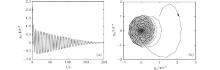
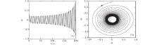
When τ = 2.9811, the time history responses and the phase diagrams of the system under different initial conditions are shown in Figs. 4 and 5. It can be seen from Figs. 4(a) and 4(b) that the time history response is stable and the phase diagram is a stable focus when the initial values are close to the equilibrium point. When the initial values are far away from the equilibrium point, the time history response is unstable and the phase diagram gradually expands away from the limit cycle in Figs. 5(a) and 5(b). When β ₁ = 0.8 and β ₂ = 0.4, the stable regions of time delay τ are shown in Table 1. The system is stable when 0 ⪁ τ < 3.4378 and a Hopf bifurcation occurs when τ passes through the critical value τ ₀ = 3.4378. We can conclude that the Hopf bifurcation is supercritical since μ ₂ > 0 and δ < 0. The phase diagram is the stable limit cycles shown in Fig. 6.

Fig. 4.

	Figure Option ViewDownloadNew Window
	Fig. 4. (a) Time history response and (b) phase diagram when the initial values are [1 × 10− 4, 1 × 10− 4, 2 × 10− 4, 2 × 10− 4] with τ = 2.9811.

Fig. 5.

	Figure Option ViewDownloadNew Window
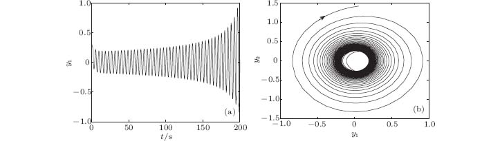	Fig. 5. (a) Time history response and (b) phase diagram when the initial values are [0.3, 0.15, 0.15, 0.3] with τ = 2.9811.

Fig. 6.

	Figure Option ViewDownloadNew Window
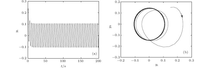	Fig. 6. (a) Time history responses and (b) phase diagram when the initial values are [0.15, 0.15, 0.2, 0.2] with τ = 3.4378.

The dynamic equation of a nonlinear electromechanical coupling transmission system is deduced according to the Lagrange– Maxwell equation and the time delay feedback is introduced to control the torsional vibration. The stable regions of time delay are obtained by using the direct method. It is found that different feedback gains correspond to different stable regions. The system can be kept stable by adjusting the feedback gains for a given time delay. The relationship between feedback gain β ₁ and the length summation of the stable regions is analyzed. Different stable regions can be obtained by changing the feedback gain. The Hopf bifurcation is studied and the explicit algorithm for determining the direction of the Hopf bifurcation and the stability of the bifurcation periodic solutions is derived by using the normal form theorem and the center manifold argument. When β ₁ = β ₂ = 1, the system produces subcritical Hopf bifurcation motion related with initial values. When β ₁ = 0.8 and β ₂ = 0.4, the Hopf bifurcation is supercritical and the limit cycles are stable. Numerical simulation results show that the subcritical bifurcation, which may cause a destructive vibration, can be effectively avoided by a reasonable selection on the delay parameters as well as the feedback gain. These results have an important theoretical significance on reducing the vibration of the electromechanical coupling transmission system. In addition, the research in our paper provides a reference for further studying the complex nonlinear dynamic behaviors of large rotary machinery.