Over the last two decades, the phenomenon of electromagnetically-induced transparency (EIT) which can eliminate the absorption at the resonant frequency of a transition by applying a control field to another transition, has attracted great attention.^{[1– 3]} The importance of EIT stems from the fact that it can enhance the nonlinear processes in the induced transparency spectral region of the medium. There are related manifestations of EIT in nonlinear optics, including giant Kerr nonlinearity, ^{[4– 7]} four-wave mixing and six-wave mixing.^{[8– 14]} The transparency is also accompanied by steep dispersion. An important application of EIT is the slowing down and even stopping of light, ^[15] while the storage and retrieval of light from an atomic ensemble has also been demonstrated.^{[16, 17]}

In the dressed-state model used to explain EIT, the so-called coupling or pump field induces dressed states, then when a probe field is tuned to the zero-field resonance frequency, the destructive interference between the excitation pathways to these states leads to the cancellation of the response at this frequency. Recently, EIT in Doppler-broadened systems has been studied by several authors, for example, the effect of Doppler broadening on the width of an EIT resonance has been investigated by Javan and co-workers.^{[18, 19]} Zhang et al. found that EIT windows are asymmetric, which come from the effect of Doppler broadening.^[20] Firstenberg et al.^[21] presented a theory of thermal motion in EIT, which includes effects of diffusion, Doppler broadening, and Dicke and Ramsey narrowing. Iftiquar et al.^[22] observed a subnatural linewidth for probe absorption in an EIT medium due to the Doppler averaging. Recently, Su et al.^[23] studied the dynamics of slow light and light storage in a Doppler-broadened EIT medium by numerically integrating the coupled Maxwell– Schrö dinger equations.

Physically, EIT is closely related to the Autler– Townes (AT) effect, ^[24] where dressed states are probed through a transition to or from a third level as a doublet excitation spectrum. Previously, we studied AT splitting in EIT-based six-wave mixing (SWM) in a Doppler-broadened system; ^{[25– 27]} the effects of Doppler broadening on the splitting were explained by a dressed-state model, whereby we analyze the velocities at which the atoms become resonant with the dressed states through Doppler frequency shifting. Based on this dressed-state model, in this paper we shall study the EIT in a Doppler-broadened cascaded three-level system. We decompose the susceptibility responsible for the EIT resonance into linear and nonlinear parts. The characteristics of EIT resonance can be understood through investigating the features of the nonlinear susceptibility.

Actually, this paper is the continuity of our previous work.^{[28– 30]} In that work we propose an alternative interpretation of EIT based on our experimental observations of the resonant stimulated Raman gain and loss spectra in a Λ -type Rb atomic vapor. Specifically, instead of the commonly accepted quantum Fano interference, the concept of Raman gain is used to explain the phenomenon of EIT. We also find that, the gain and loss can co-exist in a Doppler-broadened system, leading to polarization interference between atoms of different velocities. Obviously, the Λ -type three-level system is a special case, where the frequencies of the probe and coupling fields are almost equal. In this paper we shall consider a more general case by studying the EIT in a Doppler-broadened cascaded three-level system. It is found that the EIT resonance spectrum depends strongly on the wave-number ratio of the coupling and probe lasers. On the other hand, to obtain a Doppler-free spectrum it is necessary to have polarization interference between atoms of different velocities.

Let us consider a cascade three-level system (Fig.  1), where the states between | 0〉 and | 1〉 and between | 1〉 and | 2〉 are coupled by dipolar transitions with resonant frequencies Ω ₁ and Ω ₂ and dipole moment matrix elements μ ₁ and μ ₂, respectively. A strong coupling field (beam 2) of frequency ω ₂ resonantly couples the transition | 1〉 to | 2〉 , while a weak probe field (beam 1) of frequency ω ₁ is applied to the transition | 0〉 – | 1〉 . The effective Hamiltonian is

where Δ _i = Ω _i – ω _i is the detuning, E₁ and E₂ are the complex incident laser fields of the probe and coupling fields, respectively. The density matrix equations with relaxation terms included are given by

We are interested in the absorption of the probe beam in the presence of the coupling field. The susceptibility for the probe beam in the presence of a coupling field is given by

where G_i = μ _iE_i/ℏ is the coupling coefficients; Γ _ij is the transverse relaxation rate between states | i〉 and | j〉 . The absorption is proportional to the imaginary part of χ .

In a Doppler-broadened system, the total susceptibility is given by

Here, υ is the atomic velocity, W(υ ) = with is the mass of an atom, K is the Boltzmann’ s constant, and T is the absolute temperature, while χ (υ ) is given by Eq.  (3) with Δ _i replaced by the Doppler-shift frequency detuning and k_i is the wave vector of the i-th beam. The total susceptibility can be decomposed into linear and nonlinear parts, i.e.,

Here, and are calculated from Eq.  (4) with χ (υ ) replaced, respectively, by

Physically, originates from the two-photon coherence ρ ₂₀ induced by the probe and coupling fields. Since corresponds simply to the linear absorption in the absence of the coupling field, the characteristic of EIT resonance can be understood through investigating the features of the nonlinear susceptibility .

Fig.  1.

	Figure Option ViewDownloadNew Window
	Fig.  1. Energy-level diagram for EIT in a cascade three-level system.

Let us consider the case in which the probe and coupling fields are counterpropagating. By setting k₁ = – k₁z and k₂ = k₂z, we have and , where ζ ₂ = k₂/k₁ is the ratio between the magnitudes of the two wave vectors. Now, we express χ ^nl(υ ) in Eq.  (7) as a function of v explicitly. In the case of ζ ₂ ≠ 1, we have

where , , , and . By solving the pole structure in Eq.  (8), i.e.,

we obtain

Here,

On the other hand, the linear susceptibility is simply given by

For ζ ₂ = 1 the two-photon transition from | 0〉 to | 2〉 does not depend on the atomic velocity, and we have

Here,

We first present numerical results for the EIT resonance and the corresponding spectrum of the nonlinear susceptibility . Let us consider a Doppler-broadened system with parameters Γ ₁₀/k₁u = 0.02 and Γ ₂₀/Γ ₁₀ = 0.1. Figures  2– 4 present the imaginary parts of the total susceptibility χ _T (Figs.  2(a), 3(a), and 4(a)) and the nonlinear susceptibility (Figs.  2(b), 3(b), and 4(b)) versus Δ ₁ with ζ ₂ = 1.2, 1 and 0.8, respectively. The other parameters are Δ ₂/Γ ₁₀= 0 and G₂/Γ ₁₀ = 0.5 (solid curve), 2 (dashed curve), and 5 (dotted curve) for Figs.  2 and 3; and G₂/Γ ₁₀ = 20 (solid curve), 50 (dashed curve), and 80 (dotted curve) for Fig.  4. These figures indicate that in a Doppler-broadened system the EIT resonance depends not only on the strength of the coupling field but also on the ratios between the magnitudes of the wave vectors ζ ₂.

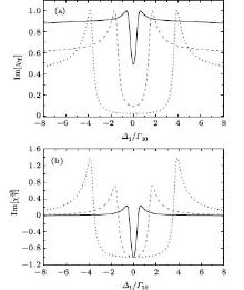
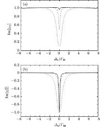
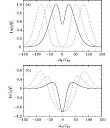
Let us first consider the case of ζ ₂ = 1.2, as shown in Fig.  2(a). On the Doppler-broadened absorption background we can see a transparency window, the width of which increases with the coupling field intensity. On the other hand, there are two absorption peaks at the edges of the EIT window. The absorption spectrum behaves quite differently when ζ ₂ = 1 [Fig.  3(a)]. Although the transparency window is still Doppler-free, no doublet structure appears in the absorption spectrum. Finally, we consider the case of ζ ₂ = 0.8 [Fig.  4(a)]. Unlike the previous cases, the spectrum is no longer Doppler free, and to obtain the doublet structure a much higher coupling field is required.

Fig.  2.

	Figure Option ViewDownloadNew Window
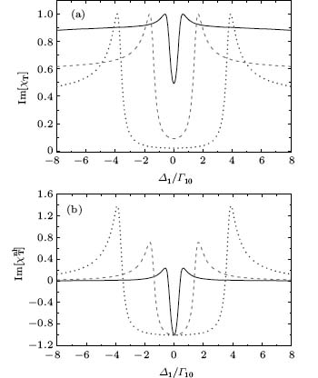	Fig.  2. Imaginary parts of (a) χ T and (b) against Δ 1 with ζ 2 = 1.2, Δ 2/Γ 10= 0, and G2/Γ 10 = 0.5 (solid curve), 2 (dashed curve), and 5 (dotted curve). In panel (a) the maximum of Im[χ T] is normalized to 1; while in panel (b) the minimum of Im[] is normalized to – 1.

Fig.  3.

	Figure Option ViewDownloadNew Window
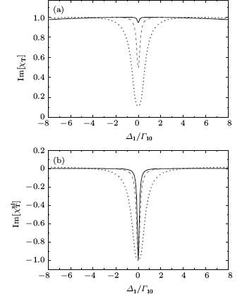	Fig.  3. Imaginary parts of (a) χ T and (b) against Δ 1 with ζ 2 = 1, Δ 2/Γ 10 = 0, and G2/Γ 10 = 0.5 (solid curve), 2 (dashed curve), and 5 (dotted curve). In panel (a) the maximum of Im[χ T] is normalized to 1; while in panel (b) the minimum of Im[] is normalized to 1.

Fig.  4.

	Figure Option ViewDownloadNew Window
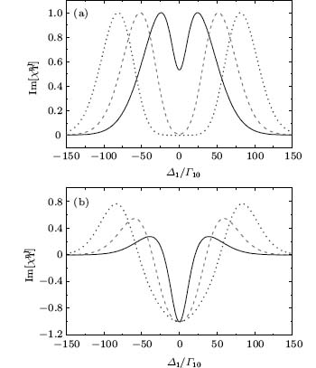	Fig.  4. Imaginary parts of (a) χ T and (b) against Δ 1 with ζ 2 = 0.8, Δ 2/Γ 10 = 0, and G2/Γ 10 = 20 (solid curve), 50 (dashed curve), and 80 (dotted curve). In panel (a) the maximum of Im[χ T] is normalized to 1; while in panel (b) the minimum of Im[] is normalized to – 1.

As mentioned before, the susceptibility for EIT can be decomposed into and [Eq.  (5)]. Since shows simply a Doppler line profile, the EIT resonance reflects mainly the characteristics of , as demonstrated in Figs.  2– 4. Let us first consider the case of ζ ₂ ≠ 1. According to Eq.  (10), there exist three poles in the nonlinear susceptibility χ ^nl(v). The values of ṽ _± and ṽ ₁ vary as we scan the probe beam, and the integral in Eq.  (4) consists mainly of the contributions of atoms with velocities v ≃ v_± and v ≃ ₁, where v_± and v₁ are the real parts of ṽ _± and ṽ ₁, respectively. For the case of v_± ≪ u, then, due to the integration, the resonance appears only when v₊ = v_– . If we ignore the relaxation rates and define Δ ₁₀ = Δ ₁/k₁ and Δ ₂₀ = (Δ ₁ +Δ ₂)/k₁(1– ζ ₂), then the resonant condition is given by

This equation is valid only when ζ ₂> 1. The two absorption peaks at the edges of the EIT window in Fig.  2 display this type of resonance. For example, for ζ ₂ = 1.2, and G₂/Γ ₁₀ = 5, the resonant peaks appear at Δ ₁/Γ ₁₀ = ± 3.7 (blue dotted curve in Fig.  2). Since the resonance originates from the contributions of atoms with velocities v = v₊ = v₋ , the spectrum is Doppler free. By contrast, the resonance at v₊ = v₋ cannot exist when ζ ₂ < 1, therefore, the spectrum is no longer Doppler free, as shown in Fig.  4. Generally speaking, the spectra of the EIT resonance and the nonlinear susceptibility in the case of ζ ₂ < 1 are similar to those in a homogeneously broadened system. However, since the spectrum is Doppler broadened, to obtain a similar spectrum a much stronger coupling field is required. Finally, let us consider the case of ζ ₂ = 1. Unlike the case of ζ ₂ ≠ 1, there are only two poles in the nonlinear susceptibility χ ^nl(v) [Eq.  (13)]. The absorption spectrum exhibits a simple dip with a Doppler-free width (Fig.  3). On the other hand, no doublet structure appears even when the coupling field is strong.

We have used Eqs.  (10) and (13) to explain the wave-vector ratio dependence of the EIT spectra. In this section we shall employ the dressed model to reveal the underlying physics of the spectra, with special emphasis on the influence of the macroscopic effects.

Let us first consider the case of ζ ₂ ≠ 1. As mentioned before, there are three poles in the nonlinear susceptibility χ ^nl(v) [Eq.  (10)]. The pole at v = ṽ ₁ reflects the transition from | 0〉 to | 1〉 in the absence of a coupling field. On the other hand, the strong coupling field beam 2 which drives the transition between | 1〉 and | 2〉 will create dressed states. In Ref. [27], we have analyzed the resonant velocities v_± at which the atoms are in resonance with the dressed states through Doppler frequency shifting. As shown in Fig.  3 in Ref. [27], when ζ ₂ < 1, the velocities v₊ and v₋ originate from the resonances of the dressed states | +〉 and | − 〉 , respectively. By contrast, we have both v₊ and v₋ from the same dressed states when ζ ₂ > 1. One consequence is that there is a gap within which no v_± exists when ζ ₂> 1. Specifically, from Eq.  (11) there is no solution for v_± in the regime .

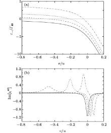
We first analyze the spectrum of the nonlinear susceptibility with ζ ₂ = 1.2 [Fig.  2(b)]. Let ɛ ₋ (v) be the eigenenergy of the lower dressed state | − 〉 of atoms with velocity v, Figures  5(a) and 5(b) present ɛ ₋ (v) and the imaginary parts of χ ^nl(v) for G₂/Γ ₁₀ = 5, Δ ₂/Γ ₁₀ = 0, ζ ₂ = 1.2, and Δ ₁/Γ ₁₀ = 3 (red dashed curve), 3.7 (black solid curve), 4 (blue dotted curve), and 5 (purple dash-dotted curve). The resonant velocities v_± correspond to the crossing points of the curves ɛ ₋ (v) with a line y = 0 (thin green solid line). There are three different regimes for v_± . As shown in Fig.  5(a), there are no solutions for v_± when Δ ₁/Γ ₁₀ = 3 (dashed curve), thus all atoms are off-resonance from the dressed states. On the other hand, due to the pole at ṽ ₁ [Eq.  (10)], Im[χ ^nl(v)] exhibits a single peak with a negative amplitude at v = Δ ₁₀ [dashed curve in Fig.  5(b)]. Atoms with velocities v ≃ v_± will contribute to the signal as Δ ₁ is tuned to the resonant frequency . Since ɛ ₋ (v) is relatively flat near the point v = v₊ = v₋ [solid curve in Fig.  5(a)], atoms in a relatively wide region of velocity will contribute to the signal at resonance. The positive peak of the solid curve in Fig.  5(b) displays this resonance. Finally, atoms of velocities v = v₊ and v = v₋ will be in resonance with the dressed state when v₊ ≠ v₋ . As a result, there are two positive peaks in the velocity dependence of Im[χ ^nl] [dotted and dash-dotted curves].

Fig.  5.

Figure Option ViewDownloadNew Window

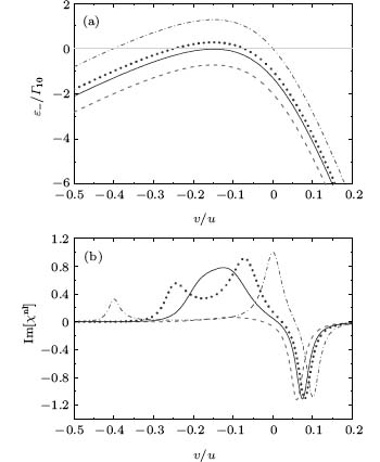Fig.  5. Velocity dependence of (a) ɛ − and (b) the imaginary part of χ nl for G2/Γ 10 = 5, Δ 2/Γ 10 = 0, ζ 2 = 1.2, and Δ 1/Γ 10 = 3 (dashed curve), 3.7 (solid curve), 4 (dotted curve), and 5 (dash-dotted curve). The resonant velocities v± correspond to the cross points of the curves ɛ − (v) with a line y = 0 (thin solid line) shown in panel (a). In panel (b) the maximum of Im[χ nl] with Δ 1/Γ 10 = 5 is normalized to 1.

Based on the characteristics of Im[χ ^nl(v)], the spectrum of the nonlinear susceptibility with ζ ₂ > 1 [Fig.  2(b)] can be understood. First, the window with negative amplitude in the spectrum of corresponds to the gap where no v_± exists. In this region, Im[] originates mainly from the contribution at the pole ṽ ₁. The amplitude of Im[] then increases sharply from negative to positive as Δ ₁ is tuned to the resonant frequency . Now let us consider the limit of . According to Eq.  (11), v_± are just the velocities of atoms at which resonant one-photon and two-photon transitions can be induced through Doppler frequency shifting in this limit. Since Im[χ ^nl(v)] at the poles ṽ ₊ and ṽ ₋ have opposite sign with that at ṽ ₁, in the case of large frequency detuning the contribution from the one-photon transition will cancel that from the pole at ṽ ₁ due to the destructive interference. As a result, the total nonlinear susceptibility Im[] originates mainly from the contribution from the two-photon transition, which decreases as the frequency detuning | Δ ₁| increases.

The spectrum of the nonlinear susceptibility with ζ ₂ < 1 is relatively easy to understand. In contrast to the case of ζ ₂ > 1, here the velocities v₊ and v₋ originate from the resonances of the dressed states | + 〉 and | − 〉 , respectively.^[27] Since there are always atoms of velocities v = v₊ and v = v₋ which are in resonance with the dressed state and so contribute to the nonlinear polarization, the spectrum exhibits a characteristic of Doppler broadening, as shown in Fig.  4.

Finally, we analyze the spectrum of the nonlinear susceptibility when ζ ₂ = 1. According to Eq.  (13), besides the pole at ṽ ₁, there exists another pole at ṽ ₂. Similar to the poles at ṽ _± , this pole is also related to the resonant velocity with the dressed state. Specifically, according to Eq.  (13) of Ref. [27], the energies of the dressed states are given by

when ζ ₂ = 1. Since the energy of the ground state | 0〉 is 0, the resonance condition for the transition from the ground to the dressed state is ɛ _± (v) = 0, and we obtain the resonant velocity

The above equation is exactly the same as Eq.  (14) when relaxation rates are ignored. Moreover, the pole at ṽ ₂ has the characteristic of a one-photon transition in the limit of large frequency detuning. Figures  6(a) and 6(b) present the dressed state energies ɛ _± (v) and the imaginary part of χ ^nl(v) for ζ ₂ = 1, G₂/Γ ₁₀ = 5, Δ ₂/Γ ₁₀ = 0, and Δ ₁/Γ ₁₀ = 0 (solid curve), 1 (dashed curve), 2 (dotted curve), and 4 (dash-dotted curve). Here again, the resonant velocities correspond to the crossing points of the curves ɛ _± (v) with a line y= 0 (thin solid line). Unlike the case of ζ ₂ ≠ 1, there is only one resonant velocity in general, while no resonant velocity exists when Δ ₁ = Δ ₂ = 0.

Let us now use Im[χ ^nl(v)] shown in Fig.  6(b) to explain the spectrum of the total nonlinear susceptibility χ _T^nl[Fig.  3(b)]. First, when Δ ₁ = Δ ₂ = 0, Im[χ ^nl(v)] exhibits a single dip (solid curve) due to the pole at ṽ ₁. When Δ ₁ becomes off-resonant, atoms with velocity v₂ will be in resonance with one of the dressed-state, so two resonant signals appear in the spectrum of Im[χ ^nl(v)]. Since Im[χ ^nl(v)] at the pole ṽ ₂ has an opposite sign to that at ṽ ₁, the destructive interference between them causes a decrease in the signal of as Δ ₁ is tuned away from the resonance. The contributions from these two poles will cancel out completely for large frequency detuning because the pole at ṽ ₂ has the characteristic of a one-photon transition in this limit. In addition, due to the absence of the gap, our model can also explain why, compared to the case of ζ ₂ > 1, there is no AT doublet even when the coupling field is strong [see the dotted curves in Figs.  2(b) and 3(b)]. Finally, we note that the destructive interference between the polarizations of atoms with different velocities can cause line narrowing of the EIT window in a Doppler-broadened system.^[22]

Fig.  6.

Figure Option ViewDownloadNew Window

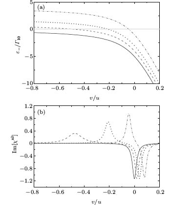Fig.  6. Velocity dependence of (a) ɛ ± and (b) the imaginary part of χ nl for ζ 2 = 1, G2/Γ 10 = 5, Δ 2/ Γ 10 = 0, and Δ 1/Γ 10 = 0 (solid curve), 1 (dashed curve), 2 (dotted curve), and 4 (dash-dotted curve). The resonant velocity v2 correspond to the cross point of the curve ɛ − (v) with a line y = 0 (thin solid line) shown in panel (a). In panel (b) the maximum of Im[χ nl] with Δ 1/Γ 10 = 4 is normalized to 1.

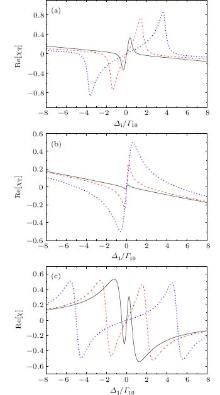
We have discussed the absorption of the EIT resonance in a Doppler-broadened system. In the following we shall make a brief discussion on the dispersion of the resonance, which will affect the propagation of the probe beam in the medium. Figures  7(a)– 7(c) present the real part of the total susceptibility χ _T with ζ ₂ = 1.2, ζ ₂ = 1 and χ respectively in a homogeneously broadened system versus Δ ₁ for Δ ₂/Γ ₁₀= 0 and G₂/Γ ₁₀ = 0.5 (solid curve), 2 (dashed curve), and 5 (dotted curve). In the homogeneously broadened system, due to the transitions to the two dressed states, the real part Re[χ ] exhibits two well-separated dispersion profiles when the coupling field is strong [dotted curve in Fig.  7(c)]. Quantum interference then occurs between these two excitation pathways when the coupling field is weak so the two transitions are overlapped, leading to a very steep variation of Re[χ ] with frequency [solid curve in Fig.  7(c)]. In contrast to the homogeneously broadened case, where Re[χ ] reflects mainly the resonant characteristic of a single atom, the EIT signal in the Doppler-broadened system involves atoms of different velocities. One important consequence is that no feature of quantum interference appears in the spectrum of Re[χ _T], as shown in Figs.  7(a) and 7(b). Instead, in the case of ζ ₂ = 1.2, we see two resonant peaks with opposite signs in amplitude, which are well separated when the coupling field is strong [dotted curve in Fig.  7(a)]. On the other hand, for ζ ₂ = 1, the spectrum of Im[χ _T] shows a simple dip [Fig.  3(a)]. Correspondingly, the spectrum of Re[χ _T] has a conventional dispersion profile but opposite in sign [Fig.  7(b)].

Fig.  7.

	Figure Option ViewDownloadNew Window
	Fig.  7. Real parts of χ T with (a) ζ 2 = 1.2, (b) ζ 2 = 1 and (c) χ in a homogeneously broadened system versus Δ 1 for Δ 2/Γ 10 = 0 and G2/Γ 10 = 0.5 (solid curve), 2 (dashed curve), and 5 (dotted curve).

In summary, we have studied the EIT resonance in a Doppler-broadened cascaded three-level system. As is well known, in a homogeneously broadened system the physics underlying the EIT resonance is the quantum interference between two excitation pathways to the dressed states, which are induced by the coupling field. By contrast, in a Doppler-broadened system the EIT resonance reflects mainly the characteristics of macroscopic effects. Specifically, the polarization interference plays a crucial role in determining the EIT resonant spectrum. For example, it is found that the EIT resonance is not only a function of the coupling laser Rabi frequency, but can also strongly depend on the wave-number ratio of the coupling and probe lasers. In the case of ζ ₂ > 1, the absorption spectrum is Doppler-free, and the EIT window is related to the existence of a gap within which no atoms can be in resonance with the dressed states through Doppler frequency shifting. On the other hand, there is no gap in the case of ζ ₂ = 1, and the absorption spectrum simply shows a narrow dip with no AT doublet even when the coupling field is very strong.