


Progress on accurate measurement of the Planck constant: Watt balance and counting atoms *
Cite this Article
Li Shi-Song, Zhang Zhong-Hua, Zhao Wei, Li Zheng-Kun, Huang Song-Ling. Progress on accurate measurement of the Planck constant: Watt balance and counting atoms * . Chinese Physics B, 2014, 24(1): 010601 
Permissions
Progress on accurate measurement of the Planck constant: Watt balance and counting atoms *
Corresponding author. E-mail: leeshisong@sina.com
Corresponding author. E-mail: zzh@nim.ac.cn
Project supported by the National Natural Science Foundation of China (Grant No. 51477160), the National Department Public Benefit Research Foundation of China (Grant No. 201010010), and the National Key Technology R&D Program of China (Grant No. 2006BAF06B01)
Abstract
The Planck constant h is one of the most significant constants in quantum physics. Recently, the precision measurement of the value of h has been a hot issue due to its important role for the establishment of both a new SI and a revised fundamental physical constant system. Up to date, two approaches, the watt balance and counting atoms, have been employed to determine the Planck constant at a level of several parts in 108. In this paper, the principle and progress on precision measurement of the Planck constant using watt balance and counting atoms at national metrology institutes are reviewed. Further improvement in determining the Planck constant and possible developments of a revised physical constant system in future are discussed.
Keyword:
06.20.–f; 06.20.Jr; 07.05.Fb; 07.10.Pz; Planck constant; watt balance; silicon sphere; Avogadro constant
1. Introduction
The Planck constant, h, is a fundamental physical constant defined originally to describe the proportionality between the energy E of a charged atomic oscillator in the black body and its frequency f, which can be expressed as E = hf.[1] Later in modern physics, some other important roles of the Planck constant were found in quantum mechanics, e.g., h is a key linkage in the quantum Hall effect (QHE), [2] the Josephson effect (JE), [3] etc. Based on its fundamental status in quantum physics, experiments determining the numeral value of the Planck constant within the international system of units (SI) have been carried out for more than one hundred years.[4]
Recently, accurate measurement of the Planck constant has been focused and will play a most important role in establishment of the new SI.[5, 6] With the rapid development of quantum physics in the last century, many macroscopic quantum phenomenons have been employed and successfully built into quantum standards for maintaining and representing SI units.[7, 8] The atomic clock is applied for high precision maintenance of the SI base unit, the second, whose measurement accuracy is at a level of at least several parts in 1016, [9] leading to wide applications in human daily life, e.g., GPS positioning, [10] meteorology, [11] navigation, [12] etc. New electrical standards, the quantum Hall resistance (QHR) standard, [13] and the Josephson voltage standard (JVS), [14] replaced the conventional artifact standards, i.e., a certain type of stable resistor and voltage cell, making the metrological accuracy for electrical quantities improved by at least two magnitudes.[15] However, the kilogram, unit of mass, is the last SI base unit that is kept by artifact, the international prototype of kilogram (IPK). The known problem for the artifact standard is its possible drift over time. For IPK, it is believed that a change of at least 50 μ g happened during one century from 1889 to 1989.[16] In order to eliminate the last artifact SI base unit, possible quantum realizations of mass have been tried. After more than thirty years of effort, the redefinition of kilogram by fixing the numerical value of the Planck constant h has been widely accepted in both metrology and physical community.[17, 18]
The new definition of the kilogram would be adopted as early as in 2018, [19] and it defines kilogram as “ kilogram, kg, is the unit of mass; its magnitude is set by fixing the numerical value of the Planck constant to be equal to exactly 6.62606X × 10− 34 J· s when it is expressed in the unit s− 1˙ m2· kg, which is equal to J· s” , [5] where X is the last few digits of h. From the recommendation of international committee for weights and measures (CIPM), the above definition can be realized only when the Planck constant is measured with a relative uncertainty of several parts in 108.
In the meantime, an accurate measurement of the Planck constant would lead to a more precise physical constant system. It can be seen from the latest evaluation report from the committee on data for science and technology (CODATA), [20] more than 99% uncertainty of some other physical constants, e.g., the Avogadro constant NA, the electron charge e, the rest mass of the electron me, the Bohr magneton μ B, and the nuclear magneton μ N, is contributed by the uncertainty component of the Planck constant. Therefore, improving the measurement accuracy of the Planck constant can synchronously reduce the uncertainties of these related constants.[21]
Accurate measurement of the Planck constant was selected as one of the most difficult scientific problems in the worldwide research in 2012, [22] since any of such approaches should combine the most precise techniques in electrical, mechanical, optical, and chemical metrology. A lot of early approaches were tried in history, e.g., the ampere balance, [23] the voltage balance, [24] the Faraday constant method, [25] etc. However, they were later proved to be metrologically limited and not persuaded further. Up to today, two ongoing approaches, watt balance, [26– 28] and counting atoms[29– 31] (also known as the X-ray crystal density method or the Avogadro project), have been proved as the most precise experiments that can measure the Planck constant at a level of several parts in 108. In this paper, progress in the watt balance experiment and the Avogadro project is reviewed. Suggestions for improving the experiments are discussed. By mapping the new SI to physics laws, possible developments of the physical constant system in future are predicted.
2. Approach principles
2.1. Watt balance principle
The origin of the watt balance was based on a conventional ampere balance experiment that was designed for absolute measurement of the SI base unit, the ampere.[23] The ampere balance was realized by balancing an electrical force and the gravity of a test mass m, written as
 |
where I1 and I2 are DC currents through the primary and secondary coils; M is the mutual inductance between two coils; and g is the acceleration due to the gravitation. The realization of the ampere balance experiment was simple; however, the measurement accuracy was limited by the largest uncertainty component arising from the geometrical factor ∂ M/∂ z. Since no direct measurement techniques were available for precision determination of the geometrical factor at that time, ∂ M/∂ z was determined by dimensional calculations according to Maxwell electromagnetic equations. Besides, the coil was a typical three-dimension system and difficult to achieve a good perfection when multi-layers were used. In reality, the coil used in ampere balance had only a few layers to ensure the geometrical uniformity for the calculation, yielding a few grams of magnetic force. As a result, it was very difficult for the ampere balance to measure a mass at kilogram level and the typical uncertainty achieved was about one part in 105.
In 1975, Kibble at National Physical Laboratory (NPL, UK) proposed a watt balance idea by dividing the experiment into two separated modes:[26] the weighing mode and the velocity mode. The weighing mode of a watt balance is operated similarly to the ampere balance with much stronger magnetic field B, expressed as
 |
where L is the coil wire length, and I is the current through the coil. In the velocity mode, the coil moves with a velocity of v in the magnetic field, yielding an induced voltage ε
 |
By combining Eqs. (2) and (3), the geometrical factor BL is eliminated, and a virtual power comparison equation, relating the electrical power to mechanical power, is obtained as
 |
In Eq. (4), the induced voltage ε is measured by a JVS linked to the Josephson effect as
 |
where f1 is a known frequency, and e is the electron charge. The current I is measured by the Josephson effect in conjunction with the quantum Hall effect as
 |
where U is the voltage drop on a resistor R in series with the coil, f2 is a known frequency, and n is an integer number. Equations (4)– (6) lead to a relation for determining the Planck constant h in the SI unit as
 |
All quantities on the right side of Eq. (7) can be precisely determined with a relative uncertainty lower than one part in 108: m is traced to IPK by mass comparators at a level of several parts in 109; [32]g is directly measured by commercial gravimeters at 10− 9 level; [33]v is determined by measuring the coil displacement using interferometers at sub-nanometer level in a total range of tens of millimeter; [34] uncertainties of f1, f2, and n are much smaller, which can be neglectful compared to 1 × 10− 9.[9] As a conclusion, on a well aligned watt balance platform, the Planck constant is expected to be determined with a relative uncertainty less than 2 × 10− 8.
2.2. Principle of counting atoms
The counting atoms, [29] also known as the X-ray crystal density (XRCD) method or the Avogadro project, is an indirect approach for precision measurement of the Planck constant. In the approach, the Avogadro constant NA is first measured by counting Si atoms in a purified silicon sphere, then the Planck constant is determined based on the product of NAh, whose value can be determined much more precise than the goal of the Planck constant determination.[20] The NAh product meets the following relationship:
 |
In Eq. (8), Ar(e) is the electron relative atomic mass with a relative uncertainty of u = 4 × 10− 10; Mu is the molar mass constant (defined as fixed constant); R∞ is the Rydberg constant, u = 5× 10− 12; c0 is the speed of light in vacuum (defined as fixed constant); α is the fine structure constant, u = 3.2 × 10− 10. According to the latest CODATA evaluation, [20] the combined measurement uncertainty for NAh is 7 × 10− 10, which is more than 60 times smaller than the uncertainty of the Planck constant u = 4.4 × 10− 8.
The history and early effort towards precision determination of the Avogadro constant by counting atoms can be found in Ref. [35]. The silicon sphere was introduced in the Avogadro project for the smaller thermal expansion coefficient and more stable surface oxide layer compared to that of other semiconductor materials, e.g., Ge. Within the approach, the natural Si crystal material was used to make the silicon spheres in the beginning; however, some metrological limits were found due to its impurity.[36] Later, the enriched 28Si single-crystal material was applied to obtain a higher degree of perfection.[37] The lattice structure of the 28Si crystal is shown in Fig. 1. Each lattice is a cube with a lattice parameter a, containing 8 28Si atoms on average. If the mole volume of 28Si single-crystal Vm is measured, the Avogadro constant then can be written as
 |
where Va is the volume of a signal 28Si atom (Va = a3/8), M0 is the mole mass of 28Si crystal, and ρ is its density.
The mole mass M0 is determined by measuring the isotope abundances of three isotopes: 28Si, 29Si, and 30Si. In reality, the isotope percentages of the crystal are measured by isotope dilution. The χ m denotes the mSi (m = 28, 29, 30) isotope percentage of the crystal, and M0 is determined as[38]
 |
The lattice parameter a is calculated from the {220} lattice-plane spacing d220 of a silicon crystal measured by the X-ray interferometer[39]
 |
The density of silicon sphere ρ is obtained by both mass and volume measurements. The mass of the silicon sphere is traced to the IPK[40] and the volume is measured by means of optical interferometers.[41] In theory, all three quantities M0, a, and ρ can be well determined with relative uncertainties of several parts in 109. The Planck constant is expected to be indirectly determined with an accuracy of 2 × 10− 8 by counting atoms in the silicon sphere.
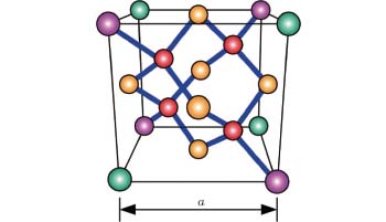 | Fig. 1. Lattice structure of the 28Si crystal. 18 28Si atoms are shown in the structure: 4 atoms (red) are inside the cube; 6 atoms (yellow) are at the centers of 6 surfaces; the other 8 atoms (pink and green) are at vertices of the cube. The average number of atoms in each lattice is N = 4+6/2+8/8 = 8. |
3. Watt balance in progress
Since the proposal in 1975, [26] the watt balance experiment was widely carried out in many national metrology institutes (NMIs) for precision determination of the Planck constant h and in future for maintaining the SI base unit, the kilogram. These metrology institutes include the NPL, the National Institute of Standards and Technology (NIST, USA), the Swiss Federal Office of Metrology (METAS, Switzerland), the Laboratoire National de mé trologie et d' essais (LNE, France), the Bureau International des Poids et Mesures (BIPM), the National Institute of Metrology (NIM, China), the National Research Council (NRC, Canada), the Measurement Standards Laboratory (MSL, New Zealand), and the Korea Research Institute of Standards and Science (KRISS, South Korea). Here the progress made at these NMIs are summarized.
3.1. NPL– NRC watt balance
The NPL is the institute that proposed and firstly practiced the watt balance idea, where the watt balance experiment was launched in 1977. In the following one decade, the first generation of watt balance, named NPL Mark I, was built in air.[42] In this approach, a beam balance was employed as the mass comparator in the weighing mode and the vertical motion stage in the velocity mode. An Fe– Co– Ni– Al permanent magnet was applied to generate a 0.7-T magnetic field. In the velocity mode, an 8-shape coil with two square segments was moved by 2 mm/s to induce a voltage of 1 V. In the weighing mode, 500 g and 1 kg were added or removed according to the current direction in coil. The first measurement result was reported in Ref. [42], h = 6.6260688(37) × 10− 34 J· s with a relative uncertainty of 5.6 × 10− 7. Later, an updated value of the Planck constant h = 6.62606821(90)× 10− 34 J· s with a relative uncertainty of 1.4 × 10− 7 was published in Ref. [43].
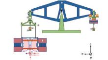
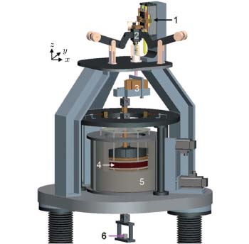
In 1990, a newly built watt balance, the NPL Mark II (shown in Fig. 2), was designed to operate in vacuum. The balance beam was preserved in the Mark II watt balance, whose beam length is 1.2 m to reduce the nonlinear motion in the velocity mode.[44] Compared to the Mark I watt balance, an important modification for Mark II was that the magnet and the coil were redesigned into horizontal circular for eliminating any linear dependence from coil movement or thermal expansion of the wire.[45] The flux of an SmCo magnet was guided to the upper and lower air gaps, generating a magnetic flux density of 0.45 T at the coil position. Two opposite series coils were buried in two air gaps. A mirror was attached to the coil former and the Michelson interferometer was used for coil position detection. The voltage drop on a 50-Ω resistor in the weighing mode and the induced voltage in the velocity mode were compared against a programmable Josephson voltage standard (PJVS) while the resistor was calibrated against a quantum Hall resistance standard through a cryogenic current comparator (CCC) bridge. The first published h = 6.62607095(44) × 10− 34 J· s was produced on NPL Mark II watt balance with a relative standard uncertainty of 6.6 × 10− 8.[45] However, after reporting the measurement, a potential mass exchange error source was identified in the weighing mode. As a result, the measurement value was adjusted to h = 6.62607123(133) × 10− 34 J· s with an expanded uncertainty of 2.0 × 10− 7.[46]
 | Fig. 2. Schematic of the NPL-NRC watt balance. 1: central knife-edge, 2: central flat, 3: balance beam, 4: end knife-edge, 5: stirrup, 6: suspension middle section, 7: lower gimbal, 8: suspension lower section, 9: test mass, 10: mass pan, 11: permanent magnet, 12: coil, 13: interferometer, 14: voice coil, 15: tare mass.[48] |
Instead of a continuous work on the new generation NPL Mark III watt balance, the NPL decided to shut down the watt balance experiment and sell the Mark II system to NRC. In 2009, the NPL Mark II watt balance was dismantled and transferred to NRC, Canada. After the reassemble, the watt balance, named NRC watt balance, was independently operated in a newly constructed laboratory. After investigating two effects, the stretching of the coil support flexures under load and the tilting effect on the balance support base due to loading and unloading the mass lift, the NRC watt balance published its first value of the Planck constant h = 6.62607063(43) × 10− 34 J· s with a relative uncertainty of 6.5 × 10− 8.[47] In 2014, an updated value of the Planck constant h = 6.62607034(12)× 10− 34 J· s, which has the smallest uncertainty of 1.9 × 10− 8 among the known h determinations, was published in Ref. [48]
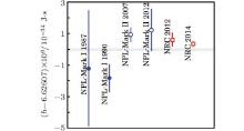
As a conclusion, all measurement results of the Planck constant h produced by NPL– NRC watt balances are summarized in Fig. 3. Although the story is a little tortuous, more than 30 years' effort has harvested the word-wide most accurate determination of the Planck constant up to date.
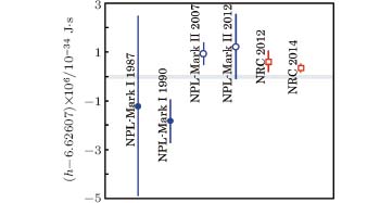 | Fig. 3. Results of h determinations by the NPL– NRC watt balance. |
3.2. NIST watt balance
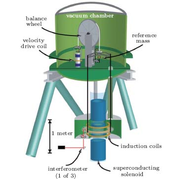
The first version of the NIST watt balance, named NIST-1, has transferred from a conventional ampere balance following the watt balance idea since 1980.[49] A rather different design for the NIST watt balance was that an electromagnetic solenoid was used to generate a radial magnetic field at the coil.[50] This realization in which the magnetic field has a 1/r contribution along the radial direction is an important conception, since in this case, the experiment would be insensitive to any linear part of both coil horizontal movements and thermal expansion, and only a second-order error should be considered. Note that this idea has been widely spread in the watt balance community, including the NPL Mark II magnet design mentioned above. The second difference of the NIST watt balance was that an aluminum wheel was used as their force comparator, which can obviously reduce the nonlinearity than that of the realization by a beam lever. In NIST-1, the solenoid generated a 2.9-mT magnetic field with 8-A DC current. In the velocity mode, a movable coil was moved with a velocity of 0.667 mm/s and an induced voltage of 20 mV was obtained. In the weighing mode, a 3.33-mA DC current passed through the movable coil and mass of 15 g was balanced. In 1989, NIST-1 produced a value of the Planck constant 6.6260704(88) × 10− 34 J· s with a relative uncertainty of 1.3 × 10− 6.[51]
Shortly after publication of NIST-1 results, an updated watt balance apparatus NIST-2 was built, in which a superconducting solenoid was added. A DC current of 5 A was passed through the new solenoid and a magnetic flux intensity of 0.1 T was obtained in an 80-mm vertical movement interval. Current of 10 mA was applied in the movable coil in the weighing mode, generating a magnetic force of 5 N to balance the gravity of a test mass of 500 g. In the velocity mode, the coil was moved at 2 mm/s to generate an induced voltage of 1 V. After years of finding misalignment errors and apparatus improvements, measurement of the Planck constant h = 6.62606891(58) × 10− 34 J· s with a relative uncertainty of 8.7 × 10− 8 was published in 1998.[34]
 | Fig. 4. Apparatus of the NIST-3 watt balance.[4] |
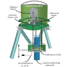
Since 1999, the NIST-2 watt balance has been updated to NIST-3(shown in Fig. 4). The main update for NIST-3 was that the watt balance was operated in vacuum instead of in air for NIST-2. In 2005, the numerical value of h = 6.62606901(34) × 10− 34 J· s with a relative uncertainty of 5.2 × 10− 8 was published.[52] After some minor improvements and reduction of the type-B uncertainty, the Planck constant h = 6.62606891(24) × − 34 J· s with a relative uncertainty of 3.6 × 10− 8 was published in 2007.[53] At that point, further improvements in reducing the measurement uncertainty was expected. However, an obvious increase of 9 × 10− 8 for the Planck constant determination was observed from March 2010 to May 2010. As part of the reason, the national mass standard K85 in United States was calibrated by the BIPM and an increase of 4 × 10⁸ was found. Towards a final determination of the Planck constant, measurements of NIST-3 watt balance were made from 2012 to 2013, yielding a value of the Planck constant h = 6.62606979(30) × 10− 34 J· s with a relative uncertainty of 4.5 × 10− 8.[54]
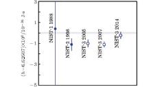
The measurement results of the Planck constant produced from the NIST watt balance have been listed in Fig. 5. No doubt that the NIST watt balance has played an importance role for decades towards the precision measurement of the Planck constant. The NIST watt balance is ongoing currently. A new watt balance, the NIST-4, which employs a permanent magnet structure similar to the magnet design of the BIPM watt balance (Section 3.5), is under construction.[55]
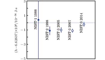 | Fig. 5. Results of h determinations by the NIST watt balance. |
3.3. METAS watt balance
The METAS watt balance started in 1997. Their first generation watt balance, the METAS Mark I, was aimed to determine the Planck constant by a compact apparatus design.[56– 58] In realization, a duel seesaw mechanism was used to move the coil in a 46-mm vertical interval. This design has advantages of avoiding both the nonlinear motion of a beam lever and the hysteresis of a knife-edge. Different from either the beam balance in NPL watt balance or the wheel design in NIST watt balance, a commercial weighing cell was employed in the METAS Mark I as the force comparator. As a rather large mechanical load was added on the mass comparator, the test mass used in the METAS Mark I watt balance was limited to 100 g. The magnetic system was designed similarly to that of the NPL Mark I watt balance. The magnetic flux of the SmCo magnet was guided by soft yoke material, generating a magnetic field of 0.56 T in the air gap. The movable coil was wound in 8-shape with 2 × 2000 turns. A typical magnetic force of 0.5 N was generated in the weighing mode when a 3 mA DC current was used. In the velocity mode, the coil was moved at 3 mm/s, generating a induced voltage of 0.5 V. In 2011, the METAS Mark I produced a final measurement of the Planck constant h = 6.6260691(20) × 10− 34 J· s with a relative uncertainty of 2.9 × 10− 7.[59]
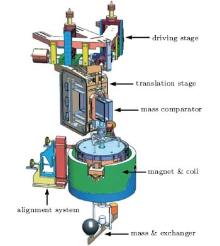
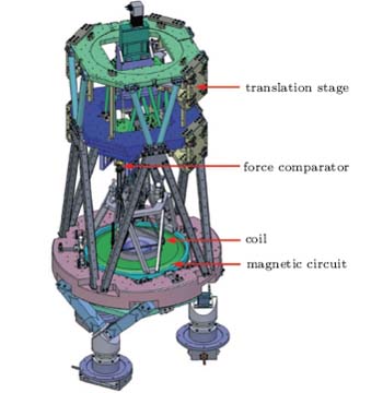
In order to determine the Planck constant with relative uncertainty of several parts in 108, a second generation watt balance, the METAS Mark II (shown in Fig. 6), is under development.[60] A driving stage based on a Sarrus linkage has been developed on the new platform. Experimental test showed that deviations from verticality in both x and y axes were smaller than 2 μ m. Moreover, a 13-hinge translation stage was built to guide the mass comparator in the velocity mode. A peak-to-peak straightness of 190 nm in the x axis and 40 nm in the y axis have been achieved in a 35-mm vertical movement interval.[61] In METAS Mark II watt balance, a magnet structure introduced by the BIPM watt balance group will be used. To reduce the large thermal effect of the SmCo magnet, a magnetic shunt compensation technique was developed in the new Mark II design. The Fe– Ni alloy shunt would be inserted into the central hole of the magnet, by changing its length, the temperature coefficient can be reduced by a factor of several hundreds. The METAS Mark II watt balance is expected to measure the Planck constant at the 10− 8 level in the near future.
 | Fig. 6. Design of the METAS watt balance Mark II.[60] |
3.4. LNE watt balance
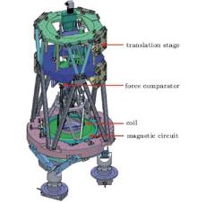
The LNE watt balance, shown in Fig. 7, began in 2001. One of the main features for the LNE watt balance is that a guiding stage is applied to move both the mass comparator and the coil.[62] This idea requires a very strong design of the guiding mechanism with minimizing motions in both the x and y directions. In realization, three flexure hinges in every 120° were chosen to move the mass comparator and the coil vertically in two planes. Experimental result showed that the horizontal motion was less than 0.5 μ m along a 75-mm vertical travel line.[63] The magnet of the LNE watt balance was designed into a one-permanent-magnet, one-coil structure.[64] The radial flux density obtained in the air gap was as high as 1 T, which has been the maximum magnetic flux density among all existing watt balances. A high magnetic field design can reduce the temperature variation due to power dissipation as well as the nonlinear magnetic errors in the weighing mode. A novel method of velocity control based on the use of a heterodyne Michelson's interferometer, a two-level translation stage, and a homemade high-frequency phase-shifting electronic circuit, has been developed and a relative uncertainty of 10− 9 over 60 mm was obtained.[65] A position sensing system based on the Gaussian beam propagation properties and the spatial modulation was applied in LNE watt balance and a resolution of 
 | Fig. 7. Design of the LNE watt balance.[63] |
3.5. BIPM watt balance
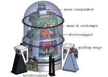
The BIPM watt balance was proposed in 2002 and launched in 2005.[71] The schematic of the BIPM watt balance is shown in Fig. 8. Several novel ideas have been practised in BIPM watt balance experiment. Firstly, the simultaneous measurement for the weighing and velocity modes are applied to reduce possible systematic effects that arise from time-varying magnetic flux density and coil misalignment. However, the voltage drop across the coil has an undesired resistive component, which should be eliminated. To remove the resistive voltage drop, the superconducting coil method, [72] bifilar coil method, [73] and data combination method[74] are being used. The second idea practised in the BIPM watt balance is that they use an electrostatic motor to drive a three-arm-lever lifting stage. The electrostatic motor eliminates additional magnetic fields generated from electromagnetic drives; however, the electrostatic force should be considered and well optimized. A contribution for the BIPM watt balance group is that they have presented a two-permanent-magnet, one-coil constructed magnet, which has a better self magnetic shielding than the one-permanent-magnet, two-coil structure applied in the NPL Mark II watt balance. The design later is followed by the METAS Mark II watt balance, [60] the NIST-4 watt balance, [55] the MSL watt balance, [75] and the KRISS watt balance.[76]
 | Fig. 8. Design of the BIPM watt balance. |
In realization, the BIPM watt balance employed a commercial air-compatible 10 kg weighing cell with 10 μ g resolution as the force comparator. A movable coil was set into an air gap with radial magnetic flux density of about 0.5 T. In the measurement, DC current of 1 mA was injected into the coil, generating a magnetic force of 1 N to balance a 100 g copper mass. In the meanwhile, the coil was moved with a constant velocity of 0.2 mm/s, yielding an induced voltage of 0.1 V. Experimental result showed that the simultaneous weighing and moving approach agreed with the bifilar coil technique in several parts in 107.[74] The BIPM watt balance is ongoing. Further improvements including noise reduction, dynamic alignment of the coil, vacuum operation, etc, are being carried out. The Planck constant with an uncertainty of several parts in 107 is expected to be published in 2015.
3.6. NIM joule balance
The joule balance experiment at NIM was proposed in 2006. Different from a conventional moving watt balance, the joule balance employs all static phases in the measurement.[77] In the weighing mode, the residual magnetic forces Δ f at different positions are measured. The velocity mode is replaced by the mutual inductance measurement of primary and secondary coils, and the Planck constant determination is described by a “ joule balance” as
 |
where M(z1) and M(z2) denote the mutual inductances at positions z1 and z2; I1 and I2 are the currents in the primary and secondary coils. The advantage for joule balance is that the dynamic measurement is avoided, and hence the uncertainty arising from coil movement would be reduced. However, it requires a precision measurement of the mutual inductance.
A joule balance prototype has been developed at NIM for principle verification since 2006. In the prototype, a coil system was introduced for generating magnetic force and a conventional beam balance was applied for weighing. A laser locking system including a piezoelectric crystal device was developed for the coil position control and a laser heterodyne interferometer was used to measure positions of the coil.[78] In order to measure the DC value of the coil mutual inductance, two methods, the linear extrapolation at low frequency[79] and the standard square wave compensation method, [80] have been developed. Two approaches can determine the mutual inductance with relative uncertainties of several parts in 107 and agree within 1 × 10− 6.
The coil system is suitable for mutual inductance measurement, but a rather large DC current is required in order to generate enough magnetic force. As a result, a serious heating problem for the coil system has been observed, which became the main uncertainty source of the joule balance. In the beginning, a 250 mA current was used to generate a 2 N magnetic force, yielding more than 100 W power consumption and 60 ppm uncertainty. Later the coil system was optimized into a compact one to improve the utility. In this case, a 3 N magnetic force was produced and the power of the coil was reduced to 40 W, reducing the uncertainty to about 9 ppm. The latest reported value of the Planck constant was h = 6.626104(59) × 10− 34 J· s published in 2014.[81]
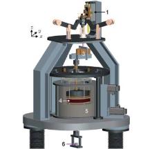
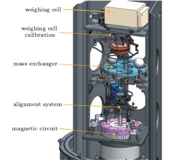
Since 2013, a new joule balance platform (shown in Fig. 9) has been under design and built. In the new system, a mass comparator will be used for weighing. The ferromagnetic coil system will be applied, which would increase the magnetic force to 5 N and reduce the power assumption to about 9 W. A vacuum system and a linear motor moving stage guiding the fixed coil are under development.
 | Fig. 9. New design of the NIM joule balance. |
3.7. MSL watt balance
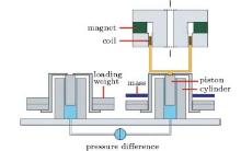
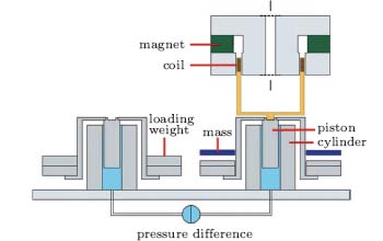
The MSL watt balance, shown in Fig. 10, is realized with several different ideas. Firstly, instead of a conventional weighing beam balance or commercial mass comparator, a twin pressure balance system was employed as the force comparator.[82] In the design, the loaded piston can be freely rotated in a close-fitting vertical cylinder, and the pressure on the piston arising from the gas compression can be several newtons. The residual force was read from a differential pressure sensor in the weighing mode. Currently, the pressure balance has achieved a 5 μ g resolution and 15 μ g uncertainty for weighing 1 kg test mass.
 | Fig. 10. Design of the MSL watt balance. |
For most watt balances, in the velocity mode, they are operated either using a constant velocity or a quasi-constant velocity with constant induced voltage. In MSL watt balance, the alter moving of the coil was designed with low frequency, e.g., 0.1– 10 Hz.[83] The advantage for this approach is that the noise band can be obviously suppressed and the signal-to-noise ratio can be improved by using Fourier analysis. In this condition, the amplitude of the induced voltage in coil is changing during the measurement, which may lead to difficulty in the voltage measurement, especially when the PJVS system is applied.
The third difference for MSL watt balance is on their magnet.[75] The magnet design is originated from the BIPM watt balance magnet with different permanent magnet locations. A ring-shaped permanent magnet and yoke arrangement is applied for generating uniform radial magnetic field in an annular gap. The design supplies higher flux concentration in the air gap and has some freedom in the choice of gap diameter. A disadvantage is that, even small gaps are added through inner and outer yokes, the systematic effect arising from the coil magnetic flux in the weighing mode should be considered carefully due to its relative low magnetic reluctance.
3.8. KRISS watt balance
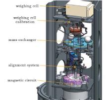
After two-year planning, KRISS became a new member of the watt balance community in 2012. Based on combination and optimization of existing watt balances techniques, the KRISS watt balance design is shown in Fig. 11.[76] The magnet is a typical two-permanent, one-coil structure, similar to the magnet of the BIPM watt balance group. The Ni– Fe alloy flux shunt is used to compensate the magnetic field change due to the temperature variations. A commercial weighing cell with capacity of 5 kg and resolution of 1 μ g from Mettler, Toledo is used in the weighing mode. A piston gauge moving stage is designed to guide the vertical motion the coil and weighing cell in the velocity mode, and a straightness of 1.2 μ m in ± 20 mm has been achieved. The first run of the KRISS watt balance is expected in 2015.
4. Progress of the Avogadro project
As discussed in Section 2.2, the Avogadro project measures the Avogadro constant NA and indirectly determines the Planck constant h based on the precision measurement of their product NAh.[20] Different from the watt balance experiment that can be carried out by an individual metrology institute, the Avogadro project is persuaded by an international collaboration between laboratories, [84] i.e., the International Avogadro Coordination (IAC). Related institutes include the Physikalisch-Technische Bundesanstalt (PTB, Germany), the National Metrology Institute of Japan (NMIJ, Japan), the METAS, the NIST, the Istituto Nazionale di Ricerca Metrologica (INRIM, Italy), the BIPM, the Institute for Reference Materials and Measurements (IRMM, Belgium), the NRC, and the National Measurement Institute (NMIA, Australia). Each institute involves at least one of the key quantities for determining the Avogadro constant NA.
The first set measurement of the Avogadro project was based on three spheres made by the natural silicon crystal, which consists an isotopic distribution of 92.2% 28Si, 4.7% 29Si, and 3.1% 30Si, respectively. The first measurement of the Planck constant h = 6.6260762(21) = 10− 34 J· s with a relative uncertainty of 3.1 × 10− 7 was published by the natural silicon crystal in 2004.[36] However, this result differs from the value obtained from the watt balance experiment by about 1 × 10− 6. It was later found by new atomic spectrometer calibrations that the difference was contributed by the isotopic distribution of natural silicon and the value of the Planck constant was corrected to be h = 6.6260681(16) × 10− 34 J· s with a reduced uncertainty of 2.4 × 10− 7.[85]
For further reducing the uncertainty caused by the mole mass measurement, a second generation silicon sphere, in which the crystal was fabricated with 99.995% 28Si, was developed.[86] The enriched 28Si material, supplied by the Institute of Chemistry of High-Purity Substances of the Russian Academy of Sciences (IChHPS-RAS) in Nizhny Novgorod and the Central Design Bureau of Machine Building (CDBMB) in Saint Petersburg, was grown into a 5-kg monocrystal (see Fig. 12) in the Leibniz-Institut fü r Kristallzü chtung (IKZ) in Berlin. Two pieces of the crystal numbered 5 and 8 were manufactured into two silicon spheres at the Australian Centre for Precision Optics (ACPO), named AVO28-S5 and AVO28-S8. The current measurement of the Avogadro project is mainly based on these two silicon spheres. Here the progress of the Avogadro project is reviewed by dividing the measurement into several aspects, i.e., measurements in mole mass, lattice parameter, mass, and volume.
4.1. Mole mass measurement
The mole mass M0 is determined following Eq. (10) by measuring the crystal sample composition of three isotopic distributions, 28Si, 29Si, and 30Si. Three methods have been developed for measuring the isotopic distribution. The gas mass spectrometry (GMS) of the SiF4 gas was applied at IRMM[38] and the GMS of a direct fluorination by BrF5 was used at the Institute of Mineral Resources (IMR, China); the isotope dilution combined with multicollector inductively coupled plasma mass spectrometry (IDMS) was used in PTB; [87] the secondary ion mass spectrometer (SIMS) using a time-of-flight mass analyser was employed in the Institute for Physics of Microstructures of the Russian Academy of Sciences (IPM-RAC).[88]
As the total isotopic distribution of 29Si and 30Si is about 0.005% , for achieving the measurement goal of 2 × 10− 8 for mole mass determination, the isotopic distribution should be measured with a relative uncertainty within 4 × 10− 4. Measurement results showed that the GMS method at IRMM and the IDMS method at PTB have achieved uncertainties less than 1 × 10− 8 for determining M0. However, the measurement uncertainties do not overlap with each other. The difference was found due to the chemical preparation of the samples.[89] By a functional analysis of adding natural silicon to the enriched silicon using the IDMS method, three methods would be consistent with each other. In the IAC determination, the data obtained by the IDMS method at PTB was used. The molar mass values obtained were 27.97697017(16) g/mol and 27.97697025(19) g/mol for AVO28-S5 and AVO28-S8, respectively.[84]
For further investigation, the difference of the mole mass determinations between PTB and IRMM, in 2011 NRC was invited to perform an independent measurement of the isotopic composition of the enriched 28Si material. The mole mass was measured to be M0 = 27.97696839(24) g/mol at NRC, [47] which obviously differed from the PTB determination. For an arbitration, the mole mass of the enriched 28Si material has also been measured at NIST and NMIJ by the IDMS method. In 2014, both the NMIJ and NIST published the measurement results, M0 (NMIJ) = 27.97697009(14) g/mol[90] and M0(NIST) = 27.976969757(92) g/mol.[91] The NMIJ and NIST results are coconscious with the PTB result and confirm the IDMS method applied by the PTB is capable of very high accuracy.
4.2. Lattice parameter measurement
In order to obtain the lattice parameter a in Eq. (9), both the absolute and relative d220 measurements have been carried out at NMIs. The first d220 measurement was taken in 1973 at NIST, [92] which was a milestone linking visible and X-ray wavelengths. Later, more accurate absolute d220 values were obtained by the combined X-ray and optical interferometer (XROI) method at PTB in Germany, [93] INRIM in Italy, [94] and NMIJ in Japan.[95] As different samples of natural silicon crystals were used in NMIs, high accuracy measurements of the relative difference of d220 were also taken at NIST[96] and PTB, [97] whose measurement data were applied for corrections during international comparisons.
As the highly enriched 28Si material is now used in order to overcome difficulties in the molar mass measurement of a natural silicon crystal, the lattice parameter of the enriched 28Si has to be remeasured. In INRIM, the XROI method has been newly developed and the travel range of the crystal analyzer was increased to many centimeters.[98] Besides, a two-crystal Laue diffractometry has been developed in NIST for absolute d220 measurement.[99] The absolute d220 measurements at INRIM and NIST, which have relative uncertainties of 3.5 × 10− 9 and 6.5 × 10− 9 respectively, agreed with each other within 2 × 10− 9.[39] Note that measurements showed the lattice parameter of the enriched silicon crystal was 1.9464(67) × 10− 6 larger than that of the natural silicon crystal, and the reported experimental value has been found by Massa et al. to be consistent with quantum-mechanics calculations.[39]
In addition, the point defects should be measured and corrected during the determination of d220. In reality, the impurity concentrations Ni were measured by infrared spectroscopy; [100] the lattice expansion and contraction coefficients β i were measured by X-ray diffraction in highly doped Si samples.[35] It is found from the relative correction value Niβ i that the deviation from homogeneous lattice spacing was less than 1 × 10− 8.
4.3. Mass measurement
The mass of the silicon crystal is measured as part of determination of the silicon crystal density ρ = m/Vm. Note that ρ in Eq. (9) should be the silicon crystal density excluding the oxide layer, hydrocarbon or other contaminations, point defects and water sorption. Therefore, m should be the sphere core mass calculated as
 |
where mt is the total mass of the sphere; ml is the mass of the sphere surface layer; and md is the mass of point defects of the crystal.
The measurement of two 28Si sphere masses mt, carried out by the BIPM, PTB and NMIJ, were compared to a 1-kg platinum-iridium (Pt/Ir) mass standard. The masses of the 28Si spheres determined in air and under vacuum showed a good agreement in the three involved laboratories, [40] and a combined relative uncertainty of 5 × 10− 9 was achieved.
The surface layer of the silicon spheres was modeled into four sub-layers, [101] named the carbonaceous contamination layer (CL), the chemisorbed water layer (CWL), the layer of metallic silicides (ML), and the pure oxide layer (OL), respectively. The mass, thickness, and chemical composition of the surface layer were characterized by several different methods, [84] including the X-ray fluorescence (XRF) analysis, the near-edge X-ray absorption fine structure (NEXAFS) spectroscopy, the X-ray reflectometry (XRR), the X-ray photoelectron spectroscopy (XPS), and the optical spectral ellipsometry (SE).[102] The CL thickness was measured by XRF with a reference sample having a 6.5-nm carbon layer, [103] and the CL mass obtained was about 14 μ g with 0.5 nm thickness. The CWL was determined by gravimetric measurement with 7.7 μ g and 0.28 nm thickness.[104] The ML mass 107.5 μ g with 0.54 nm thickness was characterized by XRF, NEXAFS, and XPS.[101] The OL was measured to be about 90 μ g with 1.4 nm thickness by XPS.[105] The combined masses of surface layer ml were determined to be 222.1(14.5) μ g and 213.6(14.4) μ g for AVO28-S5 and AVO28-S8, respectively.
The mass correction md arising from the point defects is determined as
 |
where m28 and mi are the masses of the 28Si atom and of the i-th point defect. Following Eq. (14), md corrections of 8.1(2.4) μ g and 24.3(3.3) μ g were applied for the AVO28-S5 and the AVO28-S8.
4.4. Volume measurement
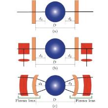
The first measurement for precision determination of the sphere volume was taken at NIST by an optical interferometer which was designed by Saunders and shown in Fig. 13(a).[106] Later a two-optical-interferometer system was developed at INRIM[107] and NMIJ, [108] as shown in Fig. 13(b), in which the reflected light from the sphere was collimated by a lens to overcome the problem due to the diffraction of the reflected light in Saunders' interferometer.[109] At PTB, a Fizeau interferometer with a spherical etalon was developed, as shown in Fig. 13(c), [110] with an advantage in analyzing the entire surface of the sphere.[111]
'> | Fig. 13. Interferometers to measure the diameter of spheres. (a) Optical configuration in Saunders' interferometer, (b) optical configuration in the NMIJ interferometer, and (c) optical configuration in the PTB interferometer. |
The measurement of the sphere diameter was differential and can be divided into two steps: 1) measuring the etalon dimension D without a sphere; and 2) measuring two gaps d1 and d2 of a sphere and the relevant plate. The sphere diameter is determined as
 |
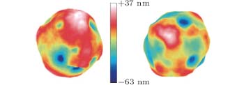
The sphere diameter measurement has been carried out in NMIA, [112] NMIJ, [113] and PTB, [114] respectively, employing the methods shown in Figs. 13(a)– 13(c). At NMIJ, single diameter values were obtained by determination of the central order of the concentric fringes. In PTB, the interference patterns are equal to the thickness fringes in a full view, which allows a complete topographical mapping of both spheres shown in Fig. 14. The comparison between NMIJ and PTB showed excellent agreement of several nanometers when d ≈ 93722.9720 μ m.
4.5. Results
In 2011, the Avogadro project published the first measurement result IAC-2011 by enriched silicon spheres.[84] The Planck constant is obtained as h = 6.62607014(20) × 10− 34 J· s with a relative uncertainty of 3.0 × 10− 8. Note that this value is between the latest results produced by the watt balance experiment, which is 3.0 × 10− 8 lower than the NRC-2014 watt balance measurement and 5.3 × 10− 8 higher than the NIST-2014 watt balance result.
By performing an independent measurement of the isotopic composition of the enriched 28Si material, when NRC produced its initial watt balance result in 2012, a determination of the Planck constant by enriched silicon sphere, h = 6.62607055(21) × 10− 34 J· s with a relative uncertainty of 3.0 × 10− 8 was also published.[47] This value is consistent with the NRC watt balance result, but 6.2 × 10− 8 higher than the IAC-2011 result.
For further checking the difference between IAC and NRC determination, the mole mass of the enriched 28Si material has also been measured at NIST and NMIJ. In 2014, NIST published its determination of the Planck constant h = 6.62607017(21) × 10− 34 J· s, [91] which is consistent with the NMIJ result h = 6.62607011(22) × 10− 34 J· s reported in the same year.[90] Both the NIST and NMIJ results agree well with the IAC-2011 result.
There is a double that the measurement result of the Avogadro project may depend on the enriched 28Si material. For further investigation of this effect, a new round of measurement is being carried out. PTB has purchased two different single 28Si crystals of 5 kg each from Russia, and four silicon spheres are under construction. It is expected that at the end of 2014, the first two silicon spheres would be ready for measurement.
5. Conclusion and discussion
5.1. Summary of the Planck constant determination
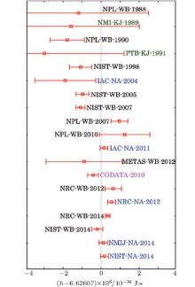
Figure 15 lists the numeral determinations of the Planck constant with relative uncertainties smaller than 1 × 10− 6.[14, 20, 47, 48, 54, 90, 91] According to CIPM 2013 recommendations, the numeral value of the Planck constant will be fixed only when the following four conditions of the approach have been achieved.
(i) At least three independent experiments, including work from watt balance and XRCD experiments, yield consistent values of the Planck constant with relative standard uncertainties not larger than 5 parts in 108.
(ii) At least one of these results should have a relative standard uncertainty not larger than 2 parts in 108.
(iii) The BIPM prototypes, the BIPM ensemble of reference mass standards, and the mass standards used in the watt balance and XRCD experiments have been compared as directly as possible with the international prototype of the kilogram.
(iv) The procedures for the future realization and dissemination of the kilogram, as described in the mise en pratique, have been validated in accordance with the principles of the CIPM Mutual Recognition Arrangement (MRA).
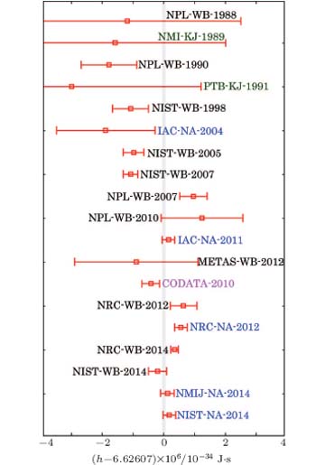 | Fig. 15. Summary of numeral determinations of the Planck constant with relative uncertainties smaller than 1 × 10− 6. KJ, WB, and NA present the result obtained from the voltage balance, the watt balance, and the Avogadro project. |
It is concluded from Fig. 15 that the NRC-WB-2014 result has achieved the CIPM recommendation (ii) with relative uncertainty of 1.9 × 10− 8; the NRC-WB-2014 result, the NIST-WB-2014 result, and the IAC-NA-2011 result have achieved the CIPM recommendation (i) with a relative uncertainty of 1.9 × 10− 8, 4.5 × 10− 8, and 3.0 × 10− 8, respectively. The mean weighted value for the Planck constant h = 6.626070235(97) × 10− 34 J· s with a relative uncertainty of 1.5 × 10− 8 is calculated based on the NRC-WB-2014 result, the NIST-WB-2014 result, and the IAC-NA-2011 result. Recommendation (iii) is being carried out and (iv) is under planing, and their results are expected to be approved in 2015 and 2017, respectively.
Although recommendations (i) and (ii) have been met, the total set of data is still inconsistent. The difference between these results is caused by certain systematic errors. During the latest years, some efforts have been paid to investigate possible systematic errors of both a watt balance and the Avogadro project (e.g., Refs. [115]– [118]). In future, on one hand, further and detailed investigation on current operated watt balance and Avogadro project should continue; on the other hand, other methods for precision measurement of the Planck constant should be encouraged.[119]
5.2. Towards a revised physical constant system
The new kilogram definition based on the fixed numeral value of the Planck constant will eliminate both time and space dependencies of an artifact standard, and hence the long-term stability of the whole SI fundamentals is improved. After the Planck constant is fixed (exact number with zero uncertainty), the uncertainties of some other constants, which are related to the Planck constant, will synchronously change following basic physical laws. As a result, this transition will also lead to a revised physical constant system. Table 1 summarizes the uncertainty change of some physical constant that are related to the Planck constant.[120]
| Table 1. Uncertainty change of some physical constants that are related to the Planck constant in the revised SI. uc and un denote the relative uncertainty in the current SI and the revised SI, respectively. |
It can be seen from Table 1 that except for a small uncertainty increase for the magnetic constant μ 0, the vacuum permittivity ε 0, and the impedance of free space Z0, the uncertainty for all the other physical constants listed has been greatly reduced. Note that during the transition of a revised physical constant system, the uncertainty of the fine structure constant α will not change. It is also notable that two typical uncertainty components after redefinition, 6.4 × 10− 10 (also most part of 7 × 10− 10) and 3.2 × 10− 10, are observed, which are mainly contributed by the fine structure constant, i.e., 2u(α ) and u(α ). Therefore, it is predicted that after the revision, the accurate measurement of the fine structure constant would be the next task towards a more precision physical constant.
5.3. Outlooks
Both the watt balance and the Avogadro project are ongoing. According to the CIPM roadmap towards a redefinition in 2018, [19] more numeral determinations of the Planck constant at NMIs will be produced in the near future. Based on the current h measurement results, we dare to say that a time for determining the Planck constant at 10− 8 level has come. For watt balance, further investigation on possible systematic effects among different NMIs should be performed in more detail to reduce both their biases and uncertainties. For the Avogadro project, a new round of measurement for the enriched 28Si should be taken to prove the data stability.
Reference
| 1 |
|
| 2 |
|
| 3 |
|
| 4 |
|
| 5 |
|
| 6 |
|
| 7 |
|
| 8 |
|
| 9 |
|
| 10 |
|
| 11 |
|
| 12 |
|
| 13 |
|
| 14 |
|
| 15 |
|
| 16 |
|
| 17 |
|
| 18 |
|
| 19 |
|
| 20 |
|
| 21 |
|
| 22 |
|
| 23 |
|
| 24 |
|
| 25 |
|
| 26 |
|
| 27 |
|
| 28 |
|
| 29 |
|
| 30 |
|
| 31 |
|
| 32 |
|
| 33 |
|
| 34 |
|
| 35 |
|
| 36 |
|
| 37 |
|
| 38 |
|
| 39 |
|
| 40 |
|
| 41 |
|
| 42 |
|
| 43 |
|
| 44 |
|
| 45 |
|
| 46 |
|
| 47 |
|
| 48 |
|
| 49 |
|
| 50 |
|
| 51 |
|
| 52 |
|
| 53 |
|
| 54 |
|
| 55 |
|
| 56 |
|
| 57 |
|
| 58 |
|
| 59 |
|
| 60 |
|
| 61 |
|
| 62 |
|
| 63 |
|
| 64 |
|
| 65 |
|
| 66 |
|
| 67 |
|
| 68 |
|
| 69 |
|
| 70 |
|
| 71 |
|
| 72 |
|
| 73 |
|
| 74 |
|
| 75 |
|
| 76 |
|
| 77 |
|
| 78 |
|
| 79 |
|
| 80 |
|
| 81 |
|
| 82 |
|
| 83 |
|
| 84 |
|
| 85 |
|
| 86 |
|
| 87 |
|
| 88 |
|
| 89 |
|
| 90 |
|
| 91 |
|
| 92 |
|
| 93 |
|
| 94 |
|
| 95 |
|
| 96 |
|
| 97 |
|
| 98 |
|
| 99 |
|
| 100 |
|
| 101 |
|
| 102 |
|
| 103 |
|
| 104 |
|
| 105 |
|
| 106 |
|
| 107 |
|
| 108 |
|
| 109 |
|
| 110 |
|
| 111 |
|
| 112 |
|
| 113 |
|
| 114 |
|
| 115 |
|
| 116 |
|
| 117 |
|
| 118 |
|
| 119 |
|
| 120 |
|