
Bayesian-MCMC-based parameter estimation of stealth aircraft RCS models
[Xia Wei†a), b)  , Dai Xiao-Xia
a), c) , Feng Yuanc) ]
, Dai Xiao-Xia|
|


†Corresponding author. E-mail: wx@uestc.edu.cn. Since March 2015, the author has been on a 12-month sabbatical leave as a visiting scholar at Stevens Institute of Technology, Hoboken, New Jersey 07030, USA.
*Project supported by the National Natural Science Foundation of China (Grant No. 61101173), the National Basic Research Program of China (Grant No. 613206), the National High Technology Research and Development Program of China (Grant No. 2012AA01A308), the State Scholarship Fund by the China Scholarship Council (CSC), and the Oversea Academic Training Funds, and University of Electronic Science and Technology of China (UESTC).
When modeling a stealth aircraft with low RCS (Radar Cross Section), conventional parameter estimation methods may cause a deviation from the actual distribution, owing to the fact that the characteristic parameters are estimated via directly calculating the statistics of RCS. The Bayesian–Markov Chain Monte Carlo (Bayesian-MCMC) method is introduced herein to estimate the parameters so as to improve the fitting accuracies of fluctuation models. The parameter estimations of the lognormal and the Legendre polynomial models are reformulated in the Bayesian framework. The MCMC algorithm is then adopted to calculate the parameter estimates. Numerical results show that the distribution curves obtained by the proposed method exhibit improved consistence with the actual ones, compared with those fitted by the conventional method. The fitting accuracy could be improved by no less than 25% for both fluctuation models, which implies that the Bayesian-MCMC method might be a good candidate among the optimal parameter estimation methods for stealth aircraft RCS models.
The radar cross section (RCS), which is an important indicator of target detection and stealth technology, represents the power gain of the electromagnetic scattering back to a radar. Since the scattering process is quite sensitive to wavelength, polarization and aspect angle etc., [1] it is of great importance to statistically model a target. Two conventional fluctuation model series are Swerling I∼ IV and Marcum models. The former are mainly applicable to traditional aircrafts, while the latter is generally applied to non-fluctuating target modeling.[2] However, the RCS could be reduced by several methods, such as shape technology, coated material technology, artificial absorbing material technology, etc.[3, 4] Therefore, it is usually difficult to statistically model the emerging aircrafts such as stealth aircrafts, high-speed flight targets, etc.[5]
In recent years, the fluctuation models with higher fitting accuracy, such as the chi-square, lognormal and Legendre polynomial models, etc., [6] have been proposed. With specific degrees of freedom, the chi-square model can be converted into Swerling I∼ IV models.[7] We herein focus on the parametric lognormal model and the nonparametric Legendre polynomial model. For the conventional lognormal model, its characteristic parameter ρ (the ratio of mean to median) is usually assumed to be greater than 1. However, in certain circumstances, for instance, when modeling a stealth target, ρ may be less than 1. Hence the complete lognormal model is proposed to tackle this problem.[8] Besides, Chen et al. illustrated that the lognormal modeling could easily result in an overestimated curve peak, especially for the aircrafts with low RCS.[9]
As for the Legendre polynomial model, the probability density of RCS reconstructed by linear combination of orthogonal polynomials yields reasonably good results.[10] However, it may be inadequate to describe the curve peaks for stealth aircraft with sharply fluctuating RCS using this model.[9] Thus, a deviation from the actual distribution may be incurred when modeling a stealth target with either the lognormal or the Legendre polynomial models. In practice, this deviation may be caused by the parameter estimation method of fluctuation models as detailed below. In the conventional methods, the characteristic parameters are estimated via calculating the statistics of RCS directly.[5] These approaches are generally suitable for parameter estimation of a traditional target with relatively well-distributed RCS. But in the case of a stealth target with low RCS property, a large error-of-fit may be caused.[11] The drawbacks of the conventional methods will be discussed in more detail later.
In order to improve the fitting accuracy of RCS, we introduce the Bayesian– Markov Chain Monte Carlo (Bayesian-MCMC) method to estimate the characteristic parameters of fluctuation models. The Bayesian-MCMC method is an effective tool to solve the posteriori estimation problem of unknown parameters. It has been successfully applied to the ocean duct inversion from radar clutter and the electromagnetic refractivity from clutter inversion, etc.[12, 13] But to the best of our knowledge, this method has not been used in estimating the unknown parameters of RCS models in existing publications. In the Bayesian-MCMC method, the parameter estimation expressions of the lognormal model and the Legendre polynomial model are derived in the Bayesian framework, and the Gibbs sampler of the MCMC method is adopted to obtain optimal parameter estimates. Simulation results show that the parameter estimates can be accurately obtained with the Bayesian-MCMC method, and the fitting accuracy can be substantially improved.
The conventional procedure to model a target is first to compute the statistics of RCS, such as the mean value, the ratio of mean to median, the kernel density function, etc. Then the statistics are substituted into the fluctuation model to approximate the probability density function (PDF) of RCS.
In this section, we will deal with the RCS modeling problem in the Bayesian framework. The expressions of the lognormal and Legendre polynomial models are treated as the posterior distribution functions of RCS variables. Combining with the Bayesian theory and the prior distribution of parameters, the parameter estimates are derived sequentially.
The classical lognormal PDF of RCS random variable σ is given by[5]
where σ 0 and 

For traditional target modeling, the value of ρ is generally assumed to be greater than 1.[8] While the RCS median σ 0 of a stealth aircraft is similar to that of a traditional aircraft; its RCS mean 
Here, we transform the lognormal problem into a normal problem to avoid calculating parameter ρ directly. Let μ and s denote the mean and standard deviation of ln σ , respectively. Thus, the basic expression of the lognormal PDF may be expressed as[10]

where ln σ is normally distributed. Equation (2) is convenient to estimate the parameters by Bayesian-MCMC method.
Now we consider the Bayesian derivation of parameter μ as a demonstration. The posterior distribution function of μ is fμ | X(μ | x), where X is a sample set of RCS variables and x is an element of X. According to the Bayesian theory, we have

where

Here, f(μ ) is the prior distribution function of μ , and it is generally assumed to be independent of the observation sample X. Besides, fX(x) is the standard factor of fμ | X(μ |x), and it is also independent of μ .[14] Thus equation (3) can be simplified into

where xi is an element of n-dimensional sample X. Therefore, the estimator of μ is
In estimating μ and s, μ can be estimated with s fixed, and vice versa.
The prior distributions of μ and s are generally specified as a normal distribution and a gamma distribution, respectively, [15] i.e., μ ∼ N(η , δ 2), s ∼ Γ (α , β ). The prior distribution of μ is
where η and δ 2 are the mean and variance of normal distribution, respectively. The prior distribution of s is

where α is the shape parameter, and β is the scale parameter.
Substituting Eqs. (2), (7), and (8) into Eq. (6), we obtain the posterior estimators


where xi is an element of X; fN(xi; s) and fN(xi; μ ) denote the basic lognormal PDF on condition that either s or μ is fixed, respectively.
In the Legendre polynomial model, the probability density of RCS is reconstructed by linear combination of orthogonal polynomials, which is given by[10]

where 

A number of numerical experiments show that satisfied fitting results could be achieved when the first 15 ∼ 25 Legendre polynomials are selected.[9] Therefore, assuming that the first m (15 ≤ m ≤ 25) polynomials are adopted, we could further obtain the posterior estimates of the polynomial coefficients a1, a2, … , am with the following procedures.
The prior distribution represents the prior knowledge about the coefficients a1, a2, … , am before the experimental observation. In practice, the low-information normal distribution is generally chosen as the prior distribution of the coefficients, [15] i.e., 
where i = 1, 2, … , m, η i and 
where fL(xi; a2, a3, … , am), … , fL(xi; a1, … , ak− 1, ak + 1, … , am), … , fL(xi; a1, a2, … , am− 1) denote respectively the PDF expressions under the condition of fixing all of the parameters except for the estimated one. Note that in practical calculation, the posterior estimates of â 1, â 2, … , â m can be solved once and for all by using Markov chains. Besides, the kernel density function of RCS data is not needed.
In the conventional method, the classical Eqs. (1) and (11) are adopted for curve fitting. Due to the low RCS property of stealth aircrafts, a large error-of-fit may be caused. In contrast, the parameter estimators in Bayesian-MCMC method are reformulated by the prior and posterior distributions of parameters. Then, the parameters estimates can be calculated by the MCMC algorithm. Finally, the estimated parameters are substituted into the basic formulae Eqs. (2) and (11) for curve fitting.
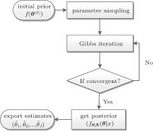
To begin with, a Markov chain is constructed by sampling. The limiting distribution of the Markov chain is the actual distribution f(θ ) of a parameter θ . With the convergent Markov chain, parameters of the fluctuation models are then estimated. The Gibbs sampling, which is one of the most popular MCMC algorithms in the Bayesian analysis, [16] is adopted herein to facilitate the calculation. The greatest advantage of MCMC method is the combination of the Monte Carlo integration with the effective sampling technique.[14] This method makes use of dynamic computer simulation technique rather than complex calculation to acquire the optimal solution.
We now consider the parameter estimation procedure by illustrating the principle of the Gibbs sampling algorithm. As shown in Subsection 2.1, the prior distributions of μ and s are μ ∼ N (η , δ 2) and s ∼ Γ (α , β ), respectively. In order to construct a Gibbs sampler for this model, we need to calculate the conditional distributions f(μ |s, X) and f(s|μ , X), and sample sequentially from these distributions. With some mathematical manipulations, [15] we could obtain

where 

Using these results, the Gibbs sampling algorithm may be summarized as follows.
Set θ = (μ , s) for the lognormal model or

for the Legendre polynomial model, and set the initial values θ (0). Then, for t = 1, … , T,
Step 1 Let θ = θ (t− 1).
Step 2 For j = 1, … , J, update θ j from θ j ∼ f(θ j| θ ∖ j, X), where θ ∖ j = (θ 1, … , θ j− 1, θ j + 1, … , θ J).
Step 3 Set θ (t) = θ for saving the generated set of values at t + 1 iteration of the algorithm.
Hence, given a particular state of the Markov chain θ (t), we generate the new parameter values in Step 2 by

So far, an iteration of the Gibbs algorithm has been completed, and the parameter set θ (t− 1) has been updated as 
In the analysis of the MCMC output, the Monte Carlo error (MC error) is adopted to measure the performance of each Markov chain. A small MC error generally corresponds to a parameter estimate with relatively high estimation precision.
The MCMC output provides us with a random sample of the type θ (1), θ (2), … , θ (t), … , θ (T). For any function G(θ ) of the interesting parameter θ , we can obtain a sample by simply considering G(θ (1)), G(θ (2)), … , G(θ (t)), … , G(θ (T)). Using these functions, we adopt the batch mean method to estimate MC error.[15] Firstly, partition the output sample into K batches (usually K = 30 or K = 50). Thus, each batch mean G̅ b(θ ) is given by

where v denotes the sample size of each batch, 
on the assumption that we keep θ (1), … , θ (T) observations. Then an estimate of the MC error is simply acquired by the standard deviation of the batch mean estimates G̅ b(θ ), [15]
The MC error changes with the batch value K (or iteration time t). When the maximum value of the MC error is less than a designated threshold ε , the sampling results can be considered to be convergent. The procedure of the Bayesian-MCMC method is summarized in Fig. 1.
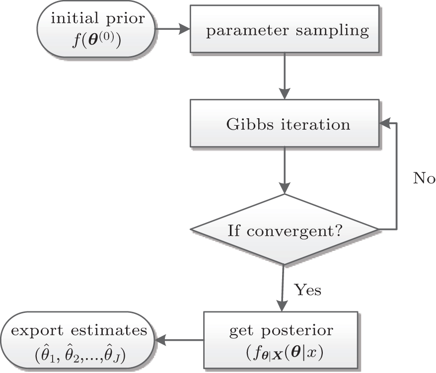 | Fig. 1. Flow chart of the Bayesian-MCMC method. |
The feasibility and accuracy of Bayesian-MCMC method for both parameter estimation and curve fitting are validated through the following numerical experiments.
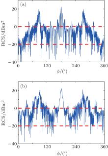
We consider two typical stealth aircraft models, namely type I and type II. Due to the complex absorbing material and its unknown electrical parameters, [17] we only consider the effect on RCS caused by the shape stealth technology. The aircraft models shown in Fig. 2 are constructed in accordance with their real size in computer aided design (CAD), and the coordinate system of stealth aircraft is also illustrated in Fig. 2(b), where ϕ and Θ denote the azimuth angle and pitch angle, respectively. Besides, the RCS data are simulated by the multilevel fast multipole method (MLFMM) in the FEKO (FEldberechnung bei Korpern mit beliebiger Oberflache). Considering the computational complexity and accuracy, this experiment is carried out at 1.3 GHz with horizontal polarization (HH), and the azimuth angle sampling interval is 0.1° (leveled off, pitch angle 0° ). The RCS sampling data of both types are shown in Fig. 3.
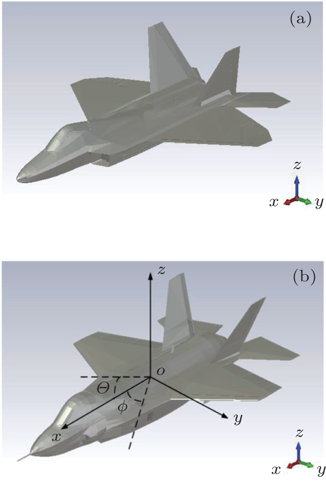 | Fig. 2. Models of stealth aircraft (a) type I and (b) type II and the coordinate system, where the head direction of an aircraft is set to be azimuth angle 0° and pitch angle 0° . |
 | Fig. 3. RCS data of (a) type I and (b) type II for different azimuth angles. The RCS data of both aircrafts are concentrated in − 20∼ 0 dB. |
Notice that the three peaks of RCS data curves correspond to the wings and tails of the aircrafts, respectively. Further, the RCS data of both aircrafts concentrate in the range of − 20 dB ∼ 0 dB, and the data of head direction gather in the range of − 20 dB ∼ 10 dB, which agree with the public data. The RCS changing trend of type II is similar to that of type I, but the mean value of RCS data of type II is less than that of type I due to its smaller physical dimension. With some direct calculations, we could find that the number of RCS data below 0 dB is up to 62.2% and 74.4% for type I and type II, respectively.
In this section, we first obtain the parameter estimates by the Bayesian-MCMC method, and then fit curves by substituting the estimated parameters into the basic functions of models. Moreover, comparisons are made between the curves fitted by the proposed method and the conventional method.
In the Bayesian-MCMC experiment, the prior distribution of each parameter is given in Section 2 and its initial value is selected according to Ref. [15]. Each Markov chain runs for 10000 iterations, and the results of the first 2000 iterations are discarded when calculating the posterior distributions. Besides, the first 20 Legendre polynomials are selected, and the threshold of the convergence criterion is 0.05. It should be noted that the RCS data hereafter are converted from logarithmic space to linear space, hence the following results are based on linear data.[5]
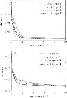
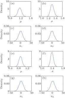
The MC errors of Markov chains and the posterior distributions of parameters for both aircrafts are illustrated in Figs. 4 and 5, respectively. It is noteworthy that only the first two parameters of the Legendre model are depicted due to a similar converging tendency of the other parameters.
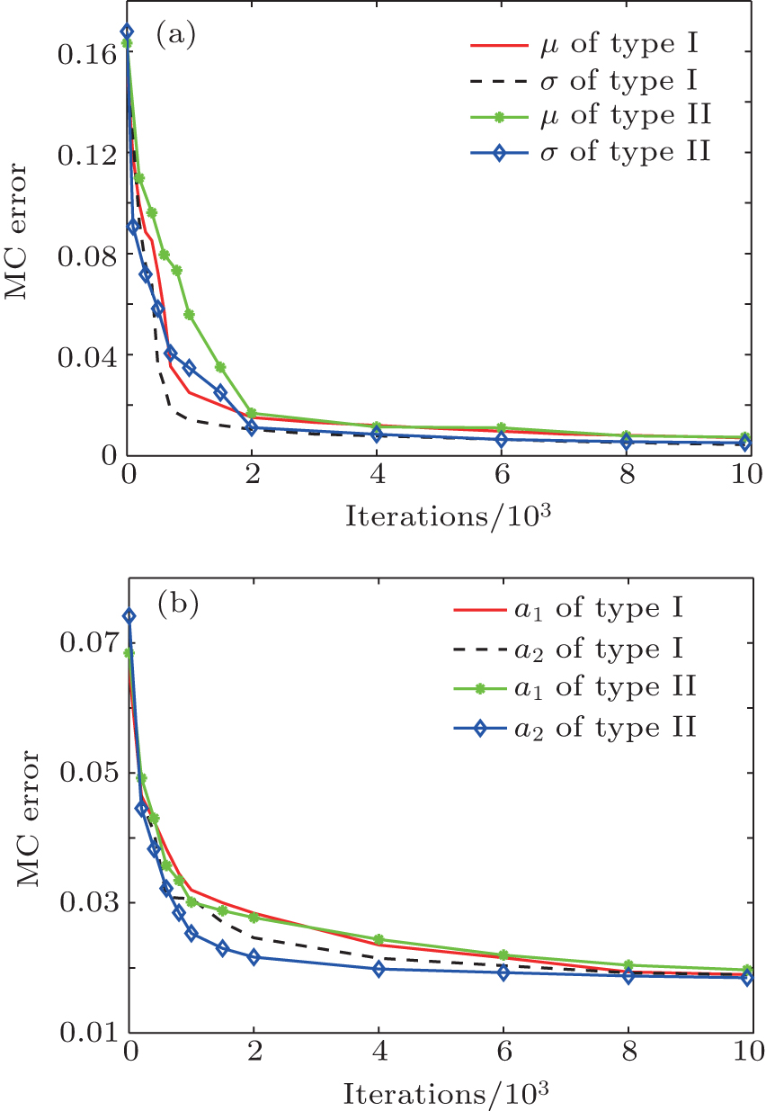 | Fig. 4. MC errors of (a) lognormal model and (b) Legendre polynomial model for both aircrafts. The number of iterations is 10000 and the MC error denotes the Monte Carlo error. |
Figure 4 shows that the MC error of Markov chains decreases rapidly as the iteration increases. The MC errors of the parameter estimates of the lognormal model converge after about 2000 iterations, while those of the Legendre polynomial model do not converge until 8000 iterations, which implies that the former estimates approximate the actual value more rapidly. In addition, the MC errors of different parameters in one model are close to the same value gradually, and the errors of the lognormal model after convergence are smaller than that of the Legendre polynomial model. It is illustrated in Fig. 5 that each posterior distribution converges towards its prior distribution (the normal distribution is the limiting distribution of the gamma distribution), and the mean value of a posterior distribution is the estimator of a parameter.
 | Fig. 5. (a) ∼ (d) Posterior distributions of parameters for type I, (e) ∼ (h) posterior distribution of parameters for type II, where panels (a), (b), (e), and (f) belong to lognormal model, panels (c), (d), (g), and (h) belong to Legendre model. |
The RCS parameter estimation results from different fluctuation models for both aircrafts are summarized in Table 1.
| Table 1. Parameter estimates and MC errors. |
As is easily observed, the estimation accuracy of the lognormal model is almost two orders of magnitude higher than that of the Legendre polynomial model with the same number of iterations. This may result from the fact that the Legendre polynomial model is essentially nonparametric, and its coefficients are not completely independent.
Here, the estimated parameters in Table 1 are substituted into the basic fluctuation models for curve fitting of Bayesian-MCMC method. Then, the fitting curves of conventional method are obtained according to Section 2. The comparisons among the fitting results are illustrated in Fig. 6.
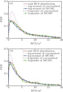
 | Fig. 6. Comparison of fitting curves for (a) type I and (b) type II, where ‘ con-method’ denotes the conventional method. |
Now, we summarize the characteristics of the RCS distributions and the fitting curves.
(i) The RCS curve peaks of both stealth aircrafts are close to the vertical axis with a narrow width, which reflects the low RCS property of stealth aircraft. Moreover, the curve peaks of type II are closer to the vertical axis due to its lower RCS.
(ii) For the curves fitted by the conventional method, the lognormal model has the drawback of overestimating the curve peak. That is because the envelope of the lognormal model is inversely proportional to the argument. The RCS mean value of type II is smaller than that of type I, and therefore the curve peak of the lognormal model for type II is higher than that of type I. On the other hand, the curves fitted by the Legendre polynomial model are more consistent with the actual distribution than those by the lognormal model. But the curve peaks cannot be appropriately estimated by the Legendre polynomial model.
(iii) For both fluctuation models, the Bayesian-MCMC method is superior to the conventional method in terms of the agreement between the fitting curves and the actual distribution of RCS. Because the proposed method estimates the parameters by constructing Markov chains rather than calculating the statistics of the RCS directly, which reduces the deviation from the actual parameters. Therefore, the estimated curve peaks exhibit improved consistence with the real peaks. In addition, the fitting precision of the curves in the large RCS region are similar to each other for both methods.
Further comparative analyses of the fitting accuracy are given below by goodness-of-fit test.
The commonly used methods of goodness-of-fit test are chi-square test, K-S test, AD (Anderson-Daring) test, etc., [18] which are mainly applicable to parametric models. While in this paper, the Legendre polynomial model is a nonparametric one so that the nonparametric test in Ref. [10] is adopted. The expression of error-of-fit is

where pi is the real probability distribution of RCS, p̂ i is the estimated probability distribution of each fluctuation model (for both methods), N0 is the number of the segments partitioned, and 
| Table 2. Errors-of-fit for both fluctuation models. |
Due to less parameters, the capability of curve fitting of the log-normal model is obviously inferior to that of the Legendre polynomial model, although the single parameter estimation accuracy of the former is superior as demonstrated in Table 1.
In terms of fitting methods, the value of error-of-fit of Bayesian-MCMC method is less than that of the conventional method for the corresponding fluctuation model. The obtained fitting accuracy amelioration is more than 25% by using the proposed method, and the most noticeable improvement is achieved for the lognormal model.
We use the Bayesian-MCMC method to improve the parameter estimation and curve fitting accuracy of fluctuation models. With the Bayesian derivation and the Markov Chain Monte Carlo estimation combined, the proposed scheme is a good way to acquire the optimal parameter estimates for both parametric and nonparametric models. The performance improvement of the proposed scheme is verified through numerical simulations. The investigation provides an alternative way to model stealth aircraft, and it is worth applying the proposed scheme to other fluctuation models to verify its universality.
The authors would like to thank Prof. Cao Chen and Dr. Huang Shuai of Electromagnetic Compatibility Laboratory, China Academy of Electronics and Information Technology, Beijing, for providing stealth aircraft models and the RCS simulation platform.
| 1 |
|
| 2 |
|
| 3 |
|
| 4 |
|
| 5 |
|
| 6 |
|
| 7 |
|
| 8 |
|
| 9 |
|
| 10 |
|
| 11 |
|
| 12 |
|
| 13 |
|
| 14 |
|
| 15 |
|
| 16 |
|
| 17 |
|
| 18 |
|