1. IntroductionSignal correlation analysis from tissue similarity (or dissimilarity) plays an important role in medical image analysis, such as tissue classification and segmentation, [1– 3] functional region localization, [3– 5] morphological evaluation, [6– 8] abnormality detection, [8– 10] and others.[11– 13]
As to similarity coefficient mapping (SCM), it is a postprocessing method and analyzes signal correlation from tissue similarity.[6] It enhances visual perceptibility of anatomical structures and helps clinical diagnosis with improved morphological evaluation. Also, it can compress a  -w magnetic resonance image series into a map which shows high image quality and non-sensitivity to the choice of reference tissues. In SCM maps, small structures, such as minor veins which are hard to distinguish from surroundings in original
  -w magnetic resonance images, are clearly observed in in vivo study and thus the accuracy of morphological evaluation of hemorrhage and pseudo-capsule of renal cancer is improved.
Wang et al.[6] has fully demonstrated how to derive the similarity map and what is the effect of the selection of the reference tissue and the echo number on map quality. However, how to interpret the SCM map is still unknown. In addition, is it probable to extract tissue dissimilarity messages based on the theory behind SCM? The purpose of this paper is to answer these two questions.
The rest of this paper is arranged in the following way. Section 2 interprets SCM from linear fitting and then extends it with an additional term to release tissue dissimilarity information into another map. Besides, the derivation of our newly proposed method and the experiment design are introduced. In Section 3, experimental results are evaluated in terms of signal-to-noise ratio (SNR) and perceived visual quality, and investigated from intra- and inter-tissue pixel intensity analysis. Discussion and conclusion of this study are presented in Sections 4 and 5, respectively.
2. Method and material2.1. Improved similarity coefficient mappingSCM measures relative signal magnitude between a tissue of interest (TOI) and a selected reference tissue. To a stationary subject, an image series

is acquired with n-echo  -w MRI and images are spatially aligned with ascending echo time (TE). Accordingly, there is a row vector of pixel intensities Vij = {Vij1, … , Vijn} for a position (i, j), while the reference signal

is constructed by averaging pixel intensities in the selected tissue region. SCM takes advantage of the mean square error (MSE) to compute the relatedness between Vij and R in the following equation,
where λ ij stands for the relative signal magnitude. Tissue dissimilarity information is valuable in tissue classification and segmentation[2] and malformation detection.[8– 10] In dynamic imaging, it was also used to uncover invisible hemodynamic responses and local pharmacokinetics.[1, 3– 5, 11, 12] In such a case, a term ε ij is added to release this kind of message in multi-echo  -w magnetic resonance image series

With known signal R and Vij, let

and

for MSEij minimization.

From Eq. (4), we get
Substituting Eq. (5) into Eq. (3), we obtain
In Eqs. (5) and (6), “ ( )” denotes the average value of a vector in ( ) and “ R' ” stands for the transpose of vector R. With these two equations, λ ij and ε ij to each signal at (i, j) can be calculated and two maps are respectively constructed in a pixel-wise computation. Please note that, in our method, the derived map from λ ij is marked as the relative magnitude map (RMM), and the map from absolute value of ε ij is marked as the residual map (RM). Also, to each image series, the derived RMM and RM make up a map pair for further investigation.
It is found that SCM and iSCM can be interpreted from the perspective of linear fitting and the theory behind them can be expressed as

and

respectively. Therefore, we can conclude that: if one signal is similar to the reference tissue signal, its value on RMM should be about 1 (it is the same interpretation to SCM) and its corresponding value on RM will be near 0. In other words, tissue similarity or dissimilarity can be quantified and crossvalidated with the generated map pair.
2.2. In vivo studyFour volunteers participated and were scanned with a 3.0 Tesla scanner (SIEMENS) with gradient-echo MRI pulse sequence (flip angle: 15° ; field of view: 220 mm × 220 mm; image matrix: 384 × 384; slice thickness: 3.0 mm; slice gap: 0.9 mm; repetition time: 200 ms). TE values range from 2.61 ms to 38.91 ms with an equal interval 3.3 ms. Four paralleling brain sections were scanned from each of these four volunteers (aged 22, 23, 25, and 29). Taken together, sixteen  -w magnetic resonance image series were collected.
2.3. Experiment designLocal cerebral-spinal fluid (CSF) and white matter (WM) tissue regions are delineated by Wei Xin-Hua (an expert radiologist from Guangzhou first Hospital, Guangzhou, China) as TOIs, and these TOIs act as the reference signal one after another. In addition, when one TOI works as the reference tissue, we will name the other one as the non-reference.
This study mainly focuses on generated map pairs from iSCM. First, the signal-to-noise ratio is quantified as SNR = μ roi/δ air, where μ roi and δ air stand for the mean value and the standard deviation value of pixel intensities in the TOI and the air region, respectively. An air region of 60 × 60 pixels is outlined in each image series and the size of TOI is 6 × 6 pixels. For each  -w magnetic resonance image series, the maximum signal-to-noise ratio (SNRmax) of each TOI is defined as the baseline for comparison. Then, tissue similarity or dissimilarity is observed from the map pair and finally interpreted from intra- and inter-tissue pixel intensity investigation.
3. Results3.1. Signal-to-noise ratio analysisThese four volunteers are indexed with V1, V2, V3, and V4 for distinction and sixteen  -w magnetic resonance image series are analyzed. For each image series, a map pair is generated from iSCM by taking the TOI of CSF or WM region to form the reference signal. For each volunteer, average SNR values of TOIs are shown in Table 1.
For each TOI in Table 1, SNRmax stands for the maximum SNR in original magnetic resonance images, SCMcsf, RMMcsf, and RMcsf indicate SNR values in the generated maps with TOI of CSF to form the reference signal, while SCMwm, RMMwm, and RMwm are SNR values in the map with TOI of WM as the reference. In addition, lower SNR values in RM are highlighted in bold.
Table 1.
Table 1.
 Table 1. Average SNR values of tissues of interest (CSF and WM) in generated maps. | TOI | SNRmax | SCMcsf | RMMcsf | RMcsf | SCMwm | RMMwm | RMwm |
|---|
| V1 | CSF | 44.80 | 141.50 | 141.51 | 2.85 | 138.90 | 138.33 | 30.22 | | WM | 59.21 | 136.64 | 136.69 | 38.46 | 140.12 | 140.13 | 1.99 | | V2 | CSF | 43.76 | 136.11 | 136.12 | 3.51 | 134.2 | 133.74 | 24.19 | | WM | 50.15 | 120.54 | 120.64 | 26.97 | 122.59 | 122.60 | 1.89 | | V3 | CSF | 40.95 | 127.30 | 127.31 | 3.07 | 125.28 | 124.81 | 21.94 | | WM | 51.66 | 123.53 | 123.61 | 22.87 | 125.61 | 125.59 | 1.93 | | V4 | CSF | 42.01 | 130.35 | 130.35 | 2.87 | 128.85 | 128.43 | 21.09 | | WM | 59.98 | 145.47 | 145.61 | 29.14 | 147.54 | 147.52 | 2.07 |
| Table 1. Average SNR values of tissues of interest (CSF and WM) in generated maps. |
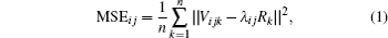
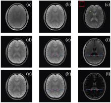
3.2. Perceived visual qualityThe third image series of the first volunteer and its derived maps are selected as a representative for visual quality analysis. In Fig. 1, [panels (a), (b), and (c)] respectively show the 1st, the 4th, and the 10th  -w magnetic resonance image, panels (d), (e), and (f) are derived maps when selecting the TOI of CSF as the reference tissue, while panels (g), (h), and (i) are maps when TOI of WM as the reference tissue. In Fig. 1(c), the delineated CSF, WM and air regions are respectively highlighted with pink, green and red squares. Pixels on blue lines in panels (e), (f), (h) and (i) are for further pixel intensity investigation, and pixels of red circle in CSF region and pixels of green sparker in WM region are for image interpretation based on the theory behind iSCM.
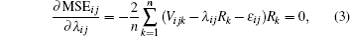
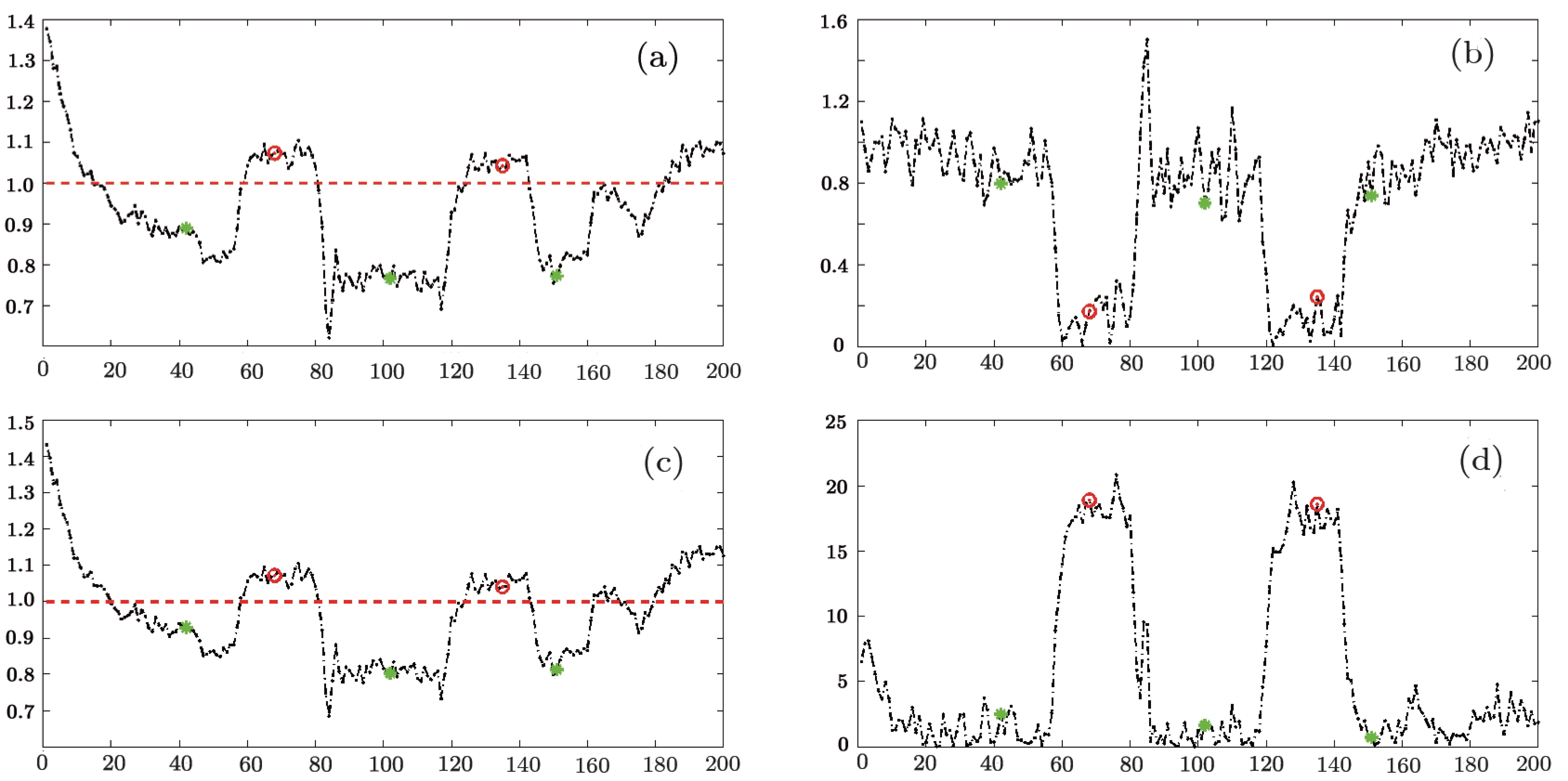
3.3. Image interpretationIntra- and inter-tissue investigation based on pixel intensity is shown in Fig. 2. In Fig. 2, black dots in panels (a), (b), (c), and (d) respectively correspond to those pixel intensities on the blue lines in Fig. 1 [panels (e), (f), (h), and (i)], and red circles and green sparkers are also in accordance with circles and sparkers in Fig. 1. The baseline of magnitude equal to 1 is indicated by red lines in panels (a) and (c).
4. DiscussionThe similarity coefficient mapping is a post-processing method and improves the morphological evaluation in  -w magnetic resonance images.[6] However, how to interpret the generated SCM map is pending. This paper firstly interpreted the theory of SCM from the perspective of linear fitting and then extended it for tissue dissimilarity messages. Finally, the improved method was validated with in vivo study and derived maps were investigated from signal-to-noise ratio and perceived visual quality, and observed from intra- and intertissue pixel intensity.
Local tissue region signal-to-noise ratio comparison is shown in Table 1, where relative magnitude map (RMM) exhibits competitive capacity as SCM in signal-to-noise ratio improvement and non-sensitivity to the reference signal, while RM demonstrates high tissue contrast. Comparing RMcsf and RMwm, it is found that the signal-to-noise ratio shows high sensitivity to the choice of the reference tissue and that the signal-to-noise ratio of non-reference tissue region is much higher than signal-to-noise ratio of the reference tissue region. For instance, to V1, when the tissue of interest of CSF performs the reference signal, the signal-to-noise of TOI in WM region in RMcsf (38.46) is about 13.5 times higher than that in CSF region in RMcsf (2.85); but when the tissue of interest of WMworks as the reference, the signal-to-noise of TOI inWM region in RMwm (1.99) is only 6.6% of that in CSF region in RMwm (30.22). This kind of sensitivity to the reference signal is also uncovered in Figs. 1 and 2.
Figure 1 shows visual image quality with one representative. When TE increases, tissue shapes, such as CSF, become much clearer and complete. With different TOIs to construct the reference signal, visual perception of SCM and RMM shows no difference and both enhance perceived quality of anatomical structures. It is found that high tissue contrast is shown in RM maps. When TOI of CSF forms the reference signal (see Fig. 1(f)), the cerebral-spinal fluid region becomes much darker than its surroundings; but when TOI of WM performs as the reference signal (see Fig. 1(i)), pixel intensities in CSF region become much higher. For image interpretation, pixels on blue lines are investigated in Fig. 2, and red circles and green sparkers are highlighted for intra- and inter-tissue pixel intensity analysis.
Medical images are the first-hand materials for image analysis and disease diagnosis[14] and the precise image interpretation plays an important role in clinical applications. As aforementioned in Subection 2.1, theoretically, if one signal is similar to the reference signal, its value on RMM is about 1, and its corresponding value on RM will be close to 0. With this understanding in mind, intra-tissue similarity and inter-tissue dissimilarity can be quantified and cross-validated.
Image interpretation is concerned in Fig. 2. From map pairs of RMM and RM, the rightness of iSCM theory is proved. When TOI of CSF work as the reference, pixel intensities of red circles in CSF region on RMM are close to 1 (see Fig. 2(a)) and on RM are near to 0 (see Fig. 2(b)); when TOI of WM is the reference, pixel intensities of green sparkers in WM region on RMM are shifted toward 1 (see Fig. 2(c)) and on RM are much closer to 0 (see Fig. 2(d)). However, it should be mentioned that, in Fig. 2(c), when taking TOI of WMas the reference tissue, green sparkers indicatingWMtissue are slightly away from the baseline. Several reasons are accountable for this kind of ambiguity. Above all, WM and grey matter are adjacent in spatial distribution in the human brain. With limited image resolution, partial volume effects play a major role and thus the reference signal is a mixture and not only purely from WM. In contrast, the cerebral-spinal fluid is more homogeneous and clear CSF shapes and boundaries lead to accurate selection. Moreover, noise, magnetic field inhomogeneity and artifacts are unavoidable in magnetic resonance images which result in the distortion of the reference signal calculation.
Another one that should be mentioned is that, it is hard to tell which one is better between SCM and RMM maps, neither from SNR comparison in Table 1 or from perceived visual quality in Fig. 1. That is because the theory behind SCM and iSCM is similar and both can be interpreted from the perspective of linear fitting. But compared to SCM, one definite advantage of iSCM lies on the RM map which shows high tissue contrast from SNR comparison (Table 1), visual perception (Fig. 1) and pixel intensity investigation (Fig. 2).
In addition, both similarity coefficient mapping and iSCM are targeted to the same tomographic slice, thus the anatomical structures in the image series should remain stationary. If relative motion occurs, spatial alignment is necessary. Meanwhile, correct selection of the reference tissue region is crucial before mapping computation and inaccurate delineation of reference tissue regions is bound to give the wrong map interpretation. In human brain study, the cerebral-spinal fluid is preferable to be the reference tissue. Our study suggests that similarity mapping techniques suppress noise, but this de-noising property does not mean the reduction of partial volume effects nor intensity in-homogeneity nor artifacts.[8]
Except for signal correlation measurements, many other techniques can be borrowed to post-process magnetic resonance image series. One simple way is to average image series. In this manner, the image quality can be improved, but higher tissue contrast is uncertain because of the intrinsic tissue difference. Another way is quantitative magnetic resonance imaging[15] which seeks to quantify fundamental biological messages and MR-inducible tissue properties, such as T2. Other methods include fuzzy clustering, principal component analysis and image compression.[16– 18]
Generally, our method belongs to the category of signal correlation measurement, but it fuses image series into two maps, i.e., RMM and RM. With the generated maps, intratissue similarity and inter-tissue dissimilarity can be quantified and cross-validated. Hence, signal investigation, organ localization, tissue classification, malformation detection and morphological evaluation can benefit from this method.


 ]
]