


Optimal satisfaction degree in energy harvesting cognitive radio networks
[Li Zan† , Liu Bo-Yang, Si Jiang-Bo, Zhou Fu-Hui]
, Liu Bo-Yang, Si Jiang-Bo, Zhou Fu-Hui]
|
|


†Corresponding author. E-mail: zanli@xidian.edu.cn
*Project supported by the National Natural Science Foundation of China (Grant No. 61301179), the Doctorial Programs Foundation of the Ministry of Education of China (Grant No. 20110203110011), and the 111 Project (Grant No. B08038).
A cognitive radio (CR) network with energy harvesting (EH) is considered to improve both spectrum efficiency and energy efficiency. A hidden Markov model (HMM) is used to characterize the imperfect spectrum sensing process. In order to maximize the whole satisfaction degree (WSD) of the cognitive radio network, a tradeoff between the average throughput of the secondary user (SU) and the interference to the primary user (PU) is analyzed. We formulate the satisfaction degree optimization problem as a mixed integer nonlinear programming (MINLP) problem. The satisfaction degree optimization problem is solved by using differential evolution (DE) algorithm. The proposed optimization problem allows the network to adaptively achieve the optimal solution based on its required quality of service (Qos). Numerical results are given to verify our analysis.
Currently, almost all the appropriate spectrum bands have been allocated to various wireless applications. The limited supply of the spectrum is becoming a bottleneck for the fast growing demands of wireless data services. Improving the spectrum efficiency is a promising solution to alleviate such a problem. However, the current fixed spectrum access strategy has little potential in improving the spectrum efficiency. Motivated by this fact, cognitive radio (CR) has been proposed in Refs. [1]– [3]. The key characteristic of CR is the ability to sense the surrounding radio environment. A lot of sensing algorithms have been proposed.[4– 7] In CR systems, secondary users (SUs) are permitted to access the bands of a primary user (PU) as long as the interference caused to the PU is acceptable. Along with the spectrum efficiency, another important area for technological advances in wireless communications is energy efficiency. It is reported that the applications and operations of information and communications technologies are estimated to contribute about 3% of global greenhouse gas emissions, and there is still an increase in the proportion.[8] Wireless devices equipped with the energy harvesting (EH) device can harvest energy from ambient sources, such as wind, solar, vibration, thermal, and even ambient radio power, which make the devices not only environmentally friendly but also self-sustaining.
As aforementioned, spectrum efficiency and energy efficiency are two key indicators of wireless systems. Combination of CR and EH is promising to the future wireless system design, which has recently drawn significant research attention. An overview of the radio frequency EH powered CR networks and the discussion of challenges that have arisen for dynamic spectrum access in these networks were provided in Ref. [9]. The theoretically achievable throughput of the SU with EH was analyzed in Ref. [10] and an optimal spectrum sensing policy that maximizes the expected total throughput subject to an energy causality constraint and a collision constraint was studied in Ref. [11]. In Refs. [12]– [15], the authors assumed that the SU is powered by EH and operates in a harvesting-sensing-transmitting fashion. The maximum throughput was achieved by optimizing the durations of saving, sensing, transmitting, [12, 13] fusion rule, [14] and SU’ s optimal cooperation strategy.[15] In Refs. [16]– [20], the partially observable Markov decision process (POMDP) was adopted to formulate and analyze the spectrum access problem with finite battery capacity of the SU in EH CR network. The design objective was to maximize the throughput of an SU. In Ref. [21], the authors determined the optimal pairing of the sensing duration and the energy detector’ s sensing threshold in order to maximize the average throughput of the SU network under the energy causality and collision constraint. A novel polarization and EH-based framework for achieving size-cost effective cooperative cognitive radio network was presented in Ref. [8]. The authors in Ref. [22] analyzed the spatial throughput of a mobile ad hoc network powered by EH using a stochastic geometry model.
All the above works focused on the optimal operation at the beginning of each time slot (harvesting or transmitting with an optimal transmit power during a slot). However, according to works in Refs. [23]– [25], activities of PUs are not random and the duration of a PU’ s activity usually lasts a number of time slots. Therefore, performing optimization at each slot not only wastes energy, but also loses opportunities for the SU to transmit signal (the SU can use the time devoted to performing optimization to transmit data). In this paper, we consider a time-slotted CR network with an EH secondary transmitter (ST). A hidden Markov model (HMM) is used to describe the imperfect spectrum sensing process. The goal of this paper is to design the sensing energy, trigger energy (the amount of the energy needed for the SU to switch into the active mode, i.e., senses the channel of the PU and decides whether to transmit or not), and the consecutive transmission slots number in order to maximize CR network’ s satisfaction degree based on the sigmoid function, subject to the energy causality and collision constraints. Increasing the sensing energy results in a waste of transmission energy, but can increase the probability of accessing the channel of the PU. Large trigger energy can increase the transmission energy, which comes at the cost of more slots needed for EH. For the consecutive transmission slots number, increasing the consecutive transmission slots number may increase the portion of the energy to transmit, but more interference causing to the PU may be imposed. Therefore, it is important to take the tradeoff among the sensing energy, trigger energy, and the consecutive transmission slots number into consideration.
The remainder of this paper is organized as follows. The system model is presented in Section 2. In Section 3, an optimization problem is formulated to obtain the optimal satisfaction degree of the CR network. Simulation results and discussion are given in Section 4. In Section 5, we conclude the paper.
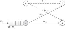
Consider a CR network consists of a pair of primary transmitters (PTs) and receivers u, v, and a pair of secondary communication nodes s, d, as depicted in Fig. 1.
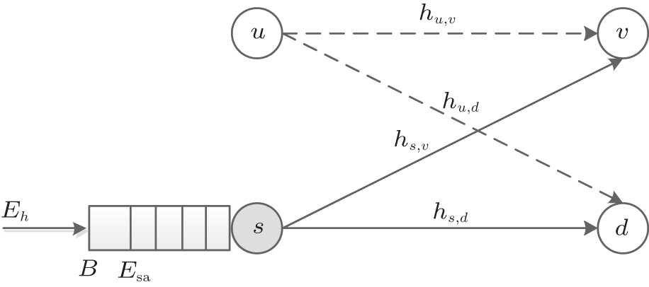 | Fig. 1. CR network model. |
The CR network is assumed to operate in a time-slotted fashion and the SU slots are synchronized to the PU slots. Let T denote the slot length and hs, v, hs, d, hu, v, hu, d denote the path losses from s to v, from s to d, from u to v, and from u to d, which are given as
where di, j is the distance between nodes i and j. κ and μ denote the pass loss constant and path loss exponent, respectively. Each receiver is affected by an additive white Gaussian noise (AWGN) with zero mean and variance 
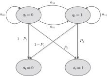
The spectrum sensing process is modeled as an HMM, as shown in Fig. 2. The status of the PU follows a discrete-time Markov process with state space X = {x1, x2}, where x1 = 0, x2 = 1. These states are hidden since they are not directly observable (due to the influence of the AWGN and the path losses). Hypotheses 


Pd = P(H1| H1) and Pf = P(H1| H0) denote the detection and false alarm probabilities, respectively. The SU senses the channel of the PU and obtains its observation sequence: 
 | Fig. 2. Spectrum sensing process. |
We assume that the ST is equipped with an energy harvester which harvests energy from ambient sources and stores the energy in a rechargeable battery with the maximum battery capacity Cmax, as shown in Fig. 1. ST can be in one of the following two modes at any given time: Harvesting mode (harvests energy from ambient sources) and active mode (senses the channel of the PU and decides whether to transmit or not). We use the Bernoulli model to illustrate the energy arrival process, which is as follows: In each time slot, SU harvests energy E with probability p. Therefore, the average energy harvesting rate is Eh = pE. The Bernoulli arrival model is simple but it still can capture the random and sporadic nature of energy arrival.[20] Similar to Ref. [22], we assume that the ST switches into the active mode only if it has Esa (trigger energy) units energy in the battery, where Esa ≤ Cmax.
An HMM can be denoted by λ = (π , A, B), where π is the initial state distribution: π = {π i}, π i = P(q1 = i), i ∈ X; A is the state transition probability matrix: A = {aij}, aij = P(qt+ 1 = j| qt = i), i, j ∈ X; B is emission probability matrix: B = {bjk}, bjk = P(ot = k| qt = j), j ∈ X, k ∈ Y. In our sensing scenario, π i = P(Hi), i ∈ X, bjk = P(Hk| Hj), j ∈ X, k ∈ Y. The parameters of the HMM are determined by solving the following optimization problem, given as[25, 26]

where p(O| λ ) is the probability of the observation sequence 

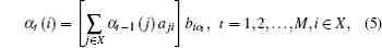

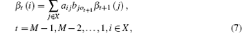
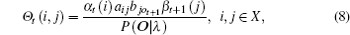


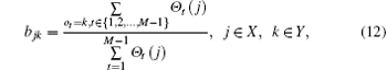
where α t (i) and β t (i) are forward and backward partial likelihoods, respectively. The iteration is initialized by setting π i = 1/2, i ∈ X, bjk = 1/2, j ∈ X, k ∈ Y, α 1 (i) = π ibio1, β M (i) = 1, i ∈ X. The iteration process might be stopped if the increase of P(O| λ ) is not larger than a threshold or the number of iterations achieves the maximum number of iteration.[26]
According to the above analysis, the complexity of the HMM training mainly concentrates on two phases: obtaining the training sequence with energy detection and the iteration process. Energy detection needs Ns multiplications and Ns − 1 additions, where Ns is the number of signal samples collected in one slot.[14] Hence, the complexity of obtaining the training sequence is M(2Ns − 1). Since the number of iterations is generally not large, the complexity of the iteration process is O(M). Therefore, the complexity of HMM training is M(2Ns − 1) + O(M).
As previously mentioned, in order to switch to the active mode, the amount of energy in the battery of the ST must achieve Esa. Since the average energy harvesting rate is Eh, the expected number of slots that the ST needs to harvest enough energy is given as

After Esa units energy is achieved, the ST switches to the active mode. In active mode, the ST first uses Es energy to sense the status of the PU and makes a decision θ t ∈ {0, 1} during one slot, where θ t = 0 denotes the PU being absent at slot t and θ t = 1 denotes the existence of the PU’ s transmission.
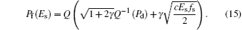
Without loss of generality, we use energy detection (ED) to execute spectrum sensing. The detection performance of SU is determined by Pd and Pf. Correct detection can protect the quality of service (Qos) of the PU. In order to guarantee a certain Qos of the PU, Pd is set to be a constant, which depends on the requirement of the PU. The Pf of ED is given by[27]

where Q(· ) is the complementary Gaussian distribution

fs is the sampling frequency of the SU. τ is the length of the sensing time and γ is the received signal-to-noise ratio (SNR) of the PU signal measured at the ST when the PU is busy, as the energy consumption is roughly linear in the number of samples, which is linear in τ . Similar to Ref. [20], we assume that τ is proportional to Es with a proportionality c. Then, equation (14) becomes
If the sensing decision made by the ST is θ t = 1, the ST will not transmit and switch to the harvesting mode at the next slot to harvest Es energy. Therefore, the expected number of slots needed for ST to harvest Es is given as
It is seen that the expected number of slots mainly comes from two parts. One is required when the PU is busy and the SU correctly detects the presence of the PU. The other is required when the PU is idle but the SU detects the presence of the PU by mistake.
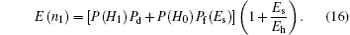
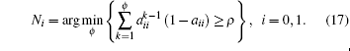
If θ t = 0, the ST will transmit its data. In this paper, we adopt a myopic strategy: The ST will exhaust all its residual energy to transmit during N consecutive slots, where N ≥ 1. As the status of the PU follows a Markov chain with 2 states, the states of the PU may maintain several consecutive slots. Let Ni denote a variable that the probability of the state xi lasting for more than Ni slots is less than 1 − ρ , where ρ is a predefined threshold. According to Ref. [25], Ni is given as
The maximum of Ni is given as

Therefore, we have 1 ≤ N ≤ Nmax. The transmit power of the ST is given as

where Pmax is the maximum transmit power of the ST. If there is sill some residual energy in the battery after N slots, the ST must release all of them to guarantee that the battery is empty at each harvesting-sensing-transmitting period, and we assume that the time for releasing the energy is negligible. Let γ p and γ s denote the target SNR for the primary user receiver and secondary user receiver, respectively.[22] Hence, the minimum transmit power of the ST is given as

The minimum Esa should afford the ST to transmit at least one slot, which means that Esa ≥ PminT. When the true state of the PU is idle, according to Eqs. (19) and (20), the data rate of the ST is given as

Note that the SU’ s data rate in Eq. (21) is normalized with W, [15] where W is the bandwidth of the channel.
Since a01 > 0, the PU may change its state several times during the N consecutive transmission slots. The PU and SU will cause interference to each other when a transmission collision appears between them. In the collision scenario, the data rate of the SU is given as

where PP is the transmit power of the PT. Meanwhile, we define the lost data rate of the PU as follows:

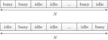
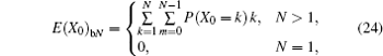
Let X0 denote the number of idle slots during N consecutive slots. As shown in Fig. 3, [25] when the current true state of the PU is busy, the expectation of X0 is given by
where m is the number of state changes during N slots and the probability p(X0 = k) is given as follows:

where

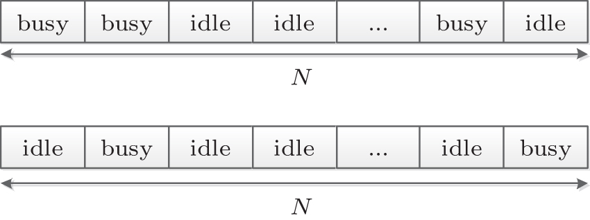 | Fig. 3. Illustration of the states changes of the PU during N consecutive slots. |
When the current true state of the PU is idle, the expectation of X0 is given by
where
where

Therefore, the expected number of idle slots in the N transmission slots is given as
The throughput of the SU in N transmission slots is given as

The ST needs to spend several slots to harvest enough energy before transmission, which results in loss of opportunities for data transmission. The performance of the SU’ s transmission cannot be evaluated by only using the throughput achieved in N transmission slots, i.e., the energy harvesting process must be considered. Hence, taking into account the energy harvesting process, we define the average throughput of the SU as

It can be seen that equation (30) is very different from that in the fixed powered scenario. Meanwhile, the interference caused to the PU is defined as

Our goal is to maximize fSU and minimize fin at the same time. From the perspective of PU, the smaller the interference caused by SU is, the better the performance of PU is. Alternatively, from the perspective of SU, the goal of SU is to achieve a transmit rate as high as possible. Thus, it is not appropriate to just simply construct an objective function as fSU − fin before all the terms are normalized. Motivated by Ref. [25], we use the sigmoid function to normalize the terms fSU and fin as


We use the weighted sum of Eqs. (32) and (33) to denote the whole satisfaction degree (WSD) of the CR network, which is given as follows:

where ω 1 and ω 2 are the weight coefficients, which reflect the requirement of the CR network. For example, if the SU’ s average throughput is more important than Qos of PU, ω 1 can be set as a large value, and vice versa.
The optimization problem to find the optimal set (Esa, Es, N) that maximizes the WSD under the energy causality and Qos constraints can be formulated as
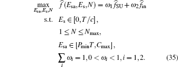
Obviously, Esa and Es are continuous variables while N is an integer variable. Therefore, the problem in Eq. (35) is a mixed-integer nonlinear programming (MINLP) problem, which is a hot topic that attracts tremendous interest. In this paper, the well-known differential evolution (DE) algorithm[28, 29] is applied to solve the optimization problem given in Eq. (35). Before using the DE algorithm, we first define 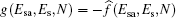
The operator ⌊ (x, y, z)⌋ in Algorithm 1 is defined as (x, y, INT[z]), where INT[z] refers to the nearest integer to z.[28] The mutation factor F is set as[29]

where F0 is a constant in the ranges from 0 to 1.
 |
In this section, we present numerical results for our proposed algorithm. Table 1 lists the simulation parameters.
| Table 1. Simulation parameters. |
Figure 4 shows the effect of the weight coefficients on the WSD with Eh = 7 and PP = 7 dB. It can be seen that the WSD increases as ω 1 increases and becomes positive when ω 1 > 0.37. This can be explained as follows. From Eqs. (32) and (33), we can see that 


 | Fig. 4. The WSD versus the weight coefficients and the target probability of detection: Eh = 7, Pp = 7 dB. |
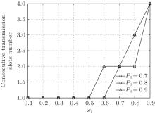
 | Fig. 5. The number of consecutive transmission slots versus the weight coefficients and the target probability of detection: Eh = 7, Pp = 7 dB. |
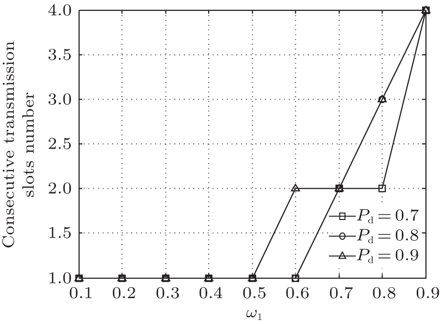
In Fig. 6, the WSD is shown with different energy harvesting rates. We can see that the WSD increases with the energy harvesting rate. It is noteworthy that as the energy harvesting rate increases, the WSD grows with a slow-down tendency, which indicates that blindly improving the energy harvesting rate is not always desirable since its contribution to the improvement of the WSD is limited in the large harvesting rate region. The reason for the phenomenon of Pd is similar to that in Fig. 4.
 | Fig. 6. The WSD versus the energy harvesting rate and the target probability of detection: ω 1 = 0.7, Pp = 7 dB. |
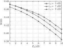
The effect of the transmit power of PU to the WSD is shown in Fig. 7 with ω 1 = 0.7, Eh = 7, and Pd = 0.9. As shown in the figure, the WSD decreases with PP. This is reasonable because higher PP leads to more interference to SU, which results in a lower 

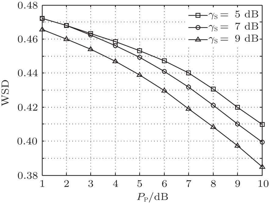 | Fig. 7. The WSD versus the transmit power of PT and the target SNR for the secondary receiver: ω 1 = 0.7, Eh = 7, Pd = 0.9. |
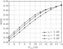
Figure 8 shows the WSD versus the maximum transmit power of ST at the target SNR for SU with ω 1 = 0.7, Eh = 7, and Pd = 0.9. As shown in the figure that the WSD increases with Pmax, which is because higher Pmax leads to a larger optimal transmit power and thus leads to a larger WSD. Moreover, it can been seen that a lower γ s leads to a higher WSD in low Pmax region and the WSD at different γ s eventually converges to the same value when Pmax is high. This can be explained as follows. When γ s is low, a lower γ s makes SU easier to successfully transmit, which leads to a higher WSD. When Pmax is high enough, the SNR corresponding to the optimal transmit power is higher than γ s.
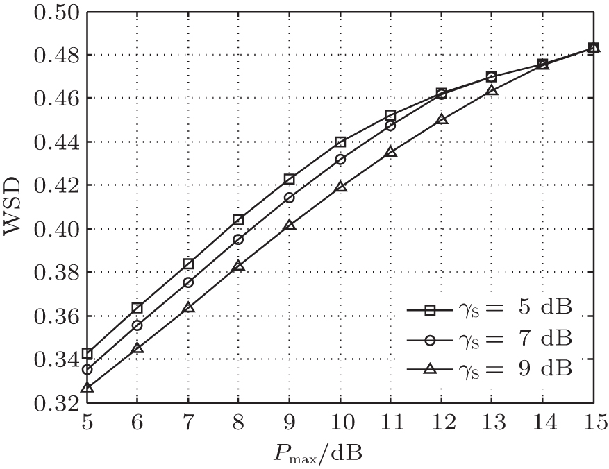 | Fig. 8. The WSD versus the maximum transmit power of ST and the target SNR for the secondary receiver: ω 1 = 0.7, Eh = 7, Pd = 0.9. |
In this paper, a CR network with EH is considered. The satisfaction degrees of SU and PU are analyzed. An HMM is used to model the sensing process. The WSD is given as a weighted sum of the two aforementioned terms, which is a function of the trigger energy, the sensing energy, and the consecutive transmission slots number. The WSD optimization is formulated as an MINLP problem and the optimal solution is obtained by DE algorithm. Simulation results confirm the analysis and show that our proposed algorithm can satisfy different requirements of the CR network by adjusting the weight coefficients.
| 1 |
|
| 2 |
|
| 3 |
|
| 4 |
|
| 5 |
|
| 6 |
|
| 7 |
|
| 8 |
|
| 9 |
|
| 10 |
|
| 11 |
|
| 12 |
|
| 13 |
|
| 14 |
|
| 15 |
|
| 16 |
|
| 17 |
|
| 18 |
|
| 19 |
|
| 20 |
|
| 21 |
|
| 22 |
|
| 23 |
|
| 24 | [Cited within:1] |
| 25 |
|
| 26 |
|
| 27 |
|
| 28 |
|
| 29 |
|