Quantum dots (QDs) are man-made structures where a controllable number of electrons are confined in an external potential.^{[1, 2]} Owing to the recent advances in semiconductor technology, it is now possible to fabricate QDs with various sizes and geometries, such as rectangular, ^[3] hexagonal, and triangular.^[4] The electronic properties of QDs have been investigated extensively because they are ideal tools to understand the electron– electron correlation effects in confined few-electron systems.^[5] QDs have also attracted considerable attention because of their application in optoelectronic device technology, such as photo-detectors, QD-based lasers, solar cells, etc.^[6]

QDs exhibit numerous interesting features by varying values of the ratio between the strength of the electron– electron interaction and the strength of the confining potential, which can also be tuned experimentally. When the strength of the external confinement is decreased, the mutual Coulomb interaction between the electrons becomes strongly dominant and the system passes from a Fermi-liquid to Wigner molecule behavior.^{[7– 10]} In a Wigner molecule regime, electrons localize in positions of classical electrons in order to minimize electron– electron interaction. According to Quantum Monte Carlo (QMC) calculations, in parabolic QDs a Wigner molecule forms below a certain critical value of electron density by showing a shell-structure and ground-state spin transitions.^[11]

Theoretically, investigation of the effect of the geometry together with the increasing Coulomb interaction on the electronic structure of the QDs gives rise to the discovery of various novel physical properties. Bryant has studied the electronic structure of rectangular quantum-well boxes containing two electrons and has observed Wigner crystallization.^[12] Creffield et al. have investigated twoelectron polygonal (square, triangular, and hexagonal) QDs by using exact diagonalization.^[13] They have observed the transition from weakly correlated Fermi-liquid behavior to strongly correlated Wigner molecule regime by examining the groundstate charge density distributions. Polygonal QDs with larger number of electrons have been studied by Rä sä nen et al. in their density functional theory (DFT) work.^[14] Recently, dependence of the ground-state spin polarization of four-electron polygonal QDs on the geometry and the size of the dot has been studied by using mean field approaches.^[15] In addition, the electronic structure of many-electron square^{[16, 17]} and rectangular^[18] QDs has been investigated with spin-DFT.

The total spin of a more-than-two electron system is a nontrivial problem in comparison with the two-electron case. Electrical controllability (without using magnetic field) of the spin state in QDs can enhance their potentiality for spin-based device applications.^[19] Several works have reported the energy spectra and charge density distribution of three-electron elliptical, ^[20] square and triangular^[21] shaped QDs at finite magnetic fields. In addition, electronic structure of threeelectron parabolic quantum dots^{[22, 23]} and quantum rings^{[19, 24]} have been studied in the absence of a magnetic field.

Unlike these studies, in the present paper we have focused on the effect of the shape of confining potential on the groundstate energy and spin configurations in quantum-dot-lithium (three-electron QD). For varying electron– electron interaction strengths at zero magnetic field, ground-state spin polarization and charge densities of hexagonal-, square-, and triangularshaped three-electron QDs are studied with the configuration interaction (CI) method.

The rest of this paper is organized as follows. In the next section we will describe the model quantum dot system and computational details of the CI method. Section 3 contains our numerical results for three-electron polygonal QDs and our conclusions are presented in Section 4.

We consider a two-dimensional (2D) quantum dot at zero magnetic field. We assume that, due to the strong confinement along the z direction, only the lowest sub-band is occupied so that electrons move on the x– y plane. Thus, in the effective mass approximation, the corresponding Hamiltonian of N-electron quantum dot system reads

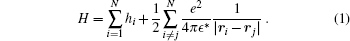
Here e, ϵ *, and r are electron charge, dielectric constant of the host semiconductor, and position of the electron, respectively. h_i is the single-particle Hamiltonian and is given as:

where p and m* are the momentum and effective mass of the electron, respectively. The external potential V(x, y), with confinement frequency ω ₀ has a form of

Here α determines the geometry of the potential, which is as taken as (2/7)cos 3γ , (1/5)cos 4γ , and (1/12)cos 6γ for triangular, ^[25] square, ^[21] and hexagonal geometries, respectively. γ corresponds to the angle between position vector (x, y) and the x axis.

It is practical to use second quantization formalism when studying many-particle systems. On the basis of selected complete and orthonormal single-particle orbitals {ϕ _i(r)}, the second quantization form of the N-electron Hamiltonian in Eq. (1) is written as

with one-body integral

and two-body integral

Here is the creation (annihilation) operator belonging to the spin orbital ϕ _i(r)σ (s) where σ (s) is the eigenfunction of z component of the spin operator with eigenvalue ± 1/2. Single-particle states {ϕ _i(r)} are chosen as eigenfunctions of the single-particle Hamiltonian. In our work single-particle states, one- and two-body integrals are calculated numerically by using the OCTOPUS code.^[26]

In the CI method the variational wave function | C〉 of the system is taken as a linear combination of Slater determinants:^[27]

where C_k are the expansion coefficients to be determined and | k〉 are the Slater determinants (SDs). N_SD is the number of SDs which are obtained by moving electrons from occupied to unoccupied states in the given orthonormal spin orbital basis. In this work, full CI is employed; i.e., all the possible SDs generated are included in the linear expansion. Inserting the variational wave function into the time-independent Schrö dinger equation yields the matrix-eigenvalue problem HC = EC, where H is the Hamiltonian matrix and C is the vector which includes the expansion coefficients.

Since the Hamiltonian of the system is spin-free, once can alternatively use Configuration State Functions (CSFs) instead of Slater determinants in Eq. (7). SDs are eigenfunctions of projected spin operator Ŝ _z only but CSFs are simultaneously eigenfunctions of the total spin Ŝ ² and Ŝ _z operators with eigenvalue S² and S_z, respectively. CSFs can be obtained by taking a proper linear combination of Slater determinants with the same eigenvalue S_z. (See Refs. [27] and [28] for more detail.) We have generated CSFs by constructing the Ŝ ² matrix in the basis of SDs with S_z eigenvalue. After diagonalization the resulting Ŝ ² matrix, the proper linear combinations are found. In the three-electron case, we keep the projection spin as S_z = 1/2 (two spin-up and one spin-down electrons), to get all the eigenstates of total spin (S = 1/2, 3/2). CSFs are primitive linear combinations of SDs and can be written as:

where b_ij are Clebsch– Gordan coefficients. We have expanded the N-electron wave function of the system, | C〉 , as a linear combination of CSFs :

The Hamiltonian matrix elements between CSFs are simply calculated by using the previously evaluated Clebsch– Gordan coefficients:

We have calculated the Hamiltonian matrix elements between SDs, 〈 j| H| j′ 〉 , analytically by using the anti-commutation relations of creation and annihilation operators.

In our model system, the total angular momentum is not quantized. Therefore, for a system with fixed number of electrons the Hamiltonian matrix becomes larger because one cannot select one-particle states with a certain angular momentum. Since the Hamiltonian matrix is symmetric and sparse, nonzero elements of the lower triangular matrix are stored with compressed sparse row format. The Hamiltonian matrix is diagonalized with Implicitly Restarted Lanczos Algorithm by using the ARPACK library.^[29] Obtained eigenvalues and eigenvectors are stored for the use in calculation of the charge density distribution of the system, n(r). We have calculated the total charge density of the system by evaluating the expectation value of the one-body operator:

among N-electron wave function:

In this section we will present our numerical results for the ground-state energies and electron densities of threeelectron hexagonal, square, and triangular quantum dots. Energies and lengths are given in units of ħ ω ₀ and l₀, respectively, which are characteristic units at zero magnetic field. The ratio of the oscillator length to the effective Bohr radius of the host material can be used to characterize the strength of the electron– electron interaction: . This dimensionless parameter can be varied by changing the strength of the confinement ω ₀. As the confinement weakens, λ becomes larger and eventually Coulomb repulsion dominates over the kinetic energy. In our work, in order to survey the ground-state properties of QDs as a function of interparticle interaction strength, we chose a wide range of λ parameters: 0 ≤ λ ≤ 10.

Mikhailov has demonstrated that the three-electron parabolic quantum dots have two significant quantum states.^[22] In the regime of weak interaction, the state S = 1/2 is the ground-state which corresponds to an unpolarized Fermi-liquid. With growing Coulomb interaction strength, a transition to S = 3/2 occurs at λ = 4.343. This spin-polarized ground-state describes the symmetric Wigner molecule in a strong interaction regime. The shape has a significant effect on the physical properties of QD^[21] and, therefore, it is noteworthy to investigate the effect of the shape of the three-electron QD on the ground-state spin transition. For that purpose, we calculate the lowest eigenstate of the three-electron hexagonal, square, and triangular QDs for different strengths of electron– electron interaction with the CI method. In all the calculations, we ensure that the desired convergence of the energies is achieved as a function of the number of single-particle orbitals (N_SP).

Table 1 shows the ground-state energies of triangular QD as a function of the number of single-particle orbitals and converged ground-state energies of the square and hexagonal QDs for varying strengths of the interaction parameter λ . In the single-particle energy spectrum of hexagonal, square, and triangular QDs, the second and third states are degenerate, as in the case of parabolic confinement. Thus, the S = 1/2 state is found to be two-fold degenerate. It can be seen from Table 1 that configurations generated from 40 single-particle orbitals are sufficient to achieve accurate results for the ground-state energy. For example, the relative error of the S = 1/2 groundstate energy for N_SP = 30 is (6.03 × 10^{− 4})% with respect to the reference energy obtained with N_SP = 40 at λ = 10. It should be noted that the CI method is the best candidate to obtain the true ground-state spin of the system because of the very small energy differences between different spin states, especially at large λ .

Table 1.

Table 1.

Table 1. CI ground-state energies (in units of ħ ω 0) of three-electron triangular QD as a function of the number of single-particle orbitals for different values of the interaction parameter λ . The last two columns represent the ground-state energies of square and hexagonal QDs for NSP = 40. λ S NSP Square Hexagonal 20 30 40 2 1/2 7.9651 7.9601 7.9573 8.1178 8.1612 3/2 8.0971 8.0956 8.0949 8.2693 8.3173 4 1/2 10.6134 10.6122 10.6116 10.9509 11.0344 3/2 10.6423 10.6412 10.6407 10.9638 11.0448 6 1/2 12.8204 12.8195 12.8194 13.3311 13.4537 3/2 12.8281 12.8274 12.8273 13.3086 13.4255 8 1/2 14.7874 14.7834 14.7834 15.4559 15.6162 3/2 14.7887 14.7858 14.7858 15.4239 15.5773 10 1/2 16.5975 16.5848 16.5847 17.4083 17.6043 3/2 16.5965 16.5855 16.5855 17.3750 17.5638

Table 1. CI ground-state energies (in units of ħ ω 0) of three-electron triangular QD as a function of the number of single-particle orbitals for different values of the interaction parameter λ . The last two columns represent the ground-state energies of square and hexagonal QDs for NSP = 40.

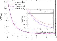
In order to better understand the influence of the shape of the QD on the ground-state spin polarization, one can focus on the spin gap, ^[30] which is defined as the energy difference between S = 3/2 and S = 1/2 spin states (Δ E = E(S = 3/2) − E(S = 1/2)). Therefore, a positive (negative) value of the spin gap corresponds to a S = 1/2 (S = 3/2) ground-state. In Fig. 1 we present the spin gap of hexagonal, square, and triangular QDs as a function of λ . The spin-gap of a parabolic QD is also given to make a comparison with polygonal geometries. The inset of Fig. 1 shows the spin gap in a smaller λ range where spin transition is seen more clearly. When the Coulomb interaction is weak (λ ≤ 2), the energy difference between the spin states is at a minimum for triangular-shaped QD which indicates an expectation for a transition to S = 3/2 state at a smaller λ than the other geometries. However, for λ ≥ 2 the spin gap decreases rapidly for all the geometries, except for the triangular geometry.

Fig. 1.

	Figure Option ViewDownloadNew Window
	Fig. 1. Energy difference between S = 3/2 and S = 1/2 states as a function of λ for different shaped QDs. The inset shows the spin gap in more detail.

In a parabolic QD the transition from S = 1/2 to S = 3/2 occurs at λ = 4.34, which is in accordance with the previous result.^[22] This interaction-induced spin transition can be explained by means of Hund’ s rule. At small λ , as a consequence of Hund’ s rule, the ground state spin of the system is S = 1/2. As λ is increased, the energy difference between single-particle states becomes very small comparing with the Coulomb interaction, which can be considered as nearly degenerate. Thus, at large λ the ground-state spin of the system is spin-polarized, S = 3/2, by obeying Hund’ s rule.^[24] In the case of hexagonal and square QDs, S = 3/2 state becomes the ground-state at λ = 4.35 and λ = 4.49, respectively. On the other hand, the situation is not the same for the triangularshaped QD because we have not observed a transition to the spin-polarized state throughout the range of λ that have been discussed. As one can see from Table 1, at large λ values the energy difference is so small that one can decide the groundstate spin from the last digit of the energy values. Our examination of the shape-dependence of the ground-state spin polarization of the three-electron quantum dot can be summarized as follows. Geometrically, the parabolic and hexagonal QDs are similar. Therefore, their transition points are found to differ only very little. The transition occurs at a higher λ value for square QDs as compared to parabolic and hexagonal QDs. When the triangular QD is considered, according to our calculations, the S = 3/2 state never becomes a ground-state. Consequently, it can be said that decreasing the number of the sides of the dot, or in other words deviation from the parabolic confinement, suppresses the polarization.

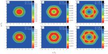
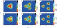
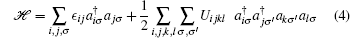
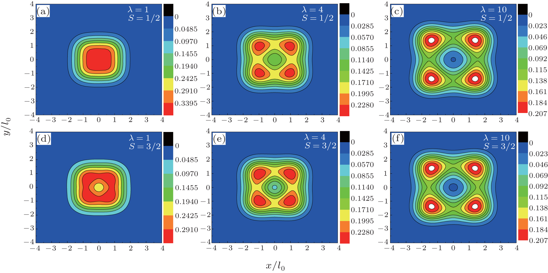
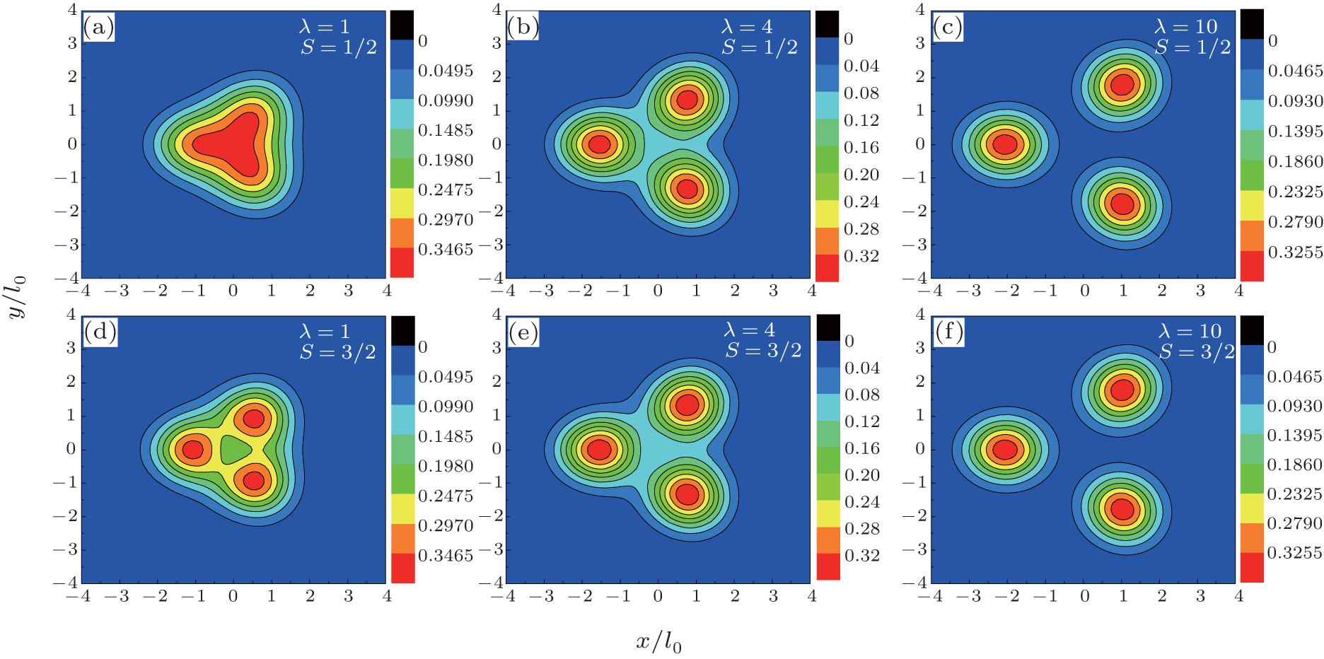
We show the total charge density plots of three electrons in hexagonal, square, and triangular QDs in Fig. 2, Fig. 3, and Fig. 4, respectively. In these figures, the first row corresponds to S = 1/2 and the second row corresponds to S = 3/2 spin state, where the interaction parameters are taken as: λ = 1 in panels (a) and (d), λ = 4 in panels (b) and (e), and λ = 10 in panels (c) and (f). Since the S = 1/2 state is two-fold degenerate, we give the average of the density of the degenerate states. The common properties of the density plots of three different shaped QDs are as follows. When the Coulomb interaction is weak (λ = 1) the electrons behave as non-interacting particles and gather at the center of the dot by reflecting the symmetry of the external potential. For λ = 4, owing to the enhanced Coulomb interaction the charge density is localized near the corners of the dot and, simultaneously, the charge density at the center decreases. With a further increment of the electron– electron interaction (λ = 10), the localization of the charge density becomes more apparent, which is a signature of a Wigner molecule formation.^[13] We have to point out that for the fully-polarized state S = 3/2, the density of spin-up and spin-down states are found to be 2/3 and 1/3 of the total charge density of the system, respectively, which is in agreement with Ref. [22].

Fig. 2.

	Figure Option ViewDownloadNew Window
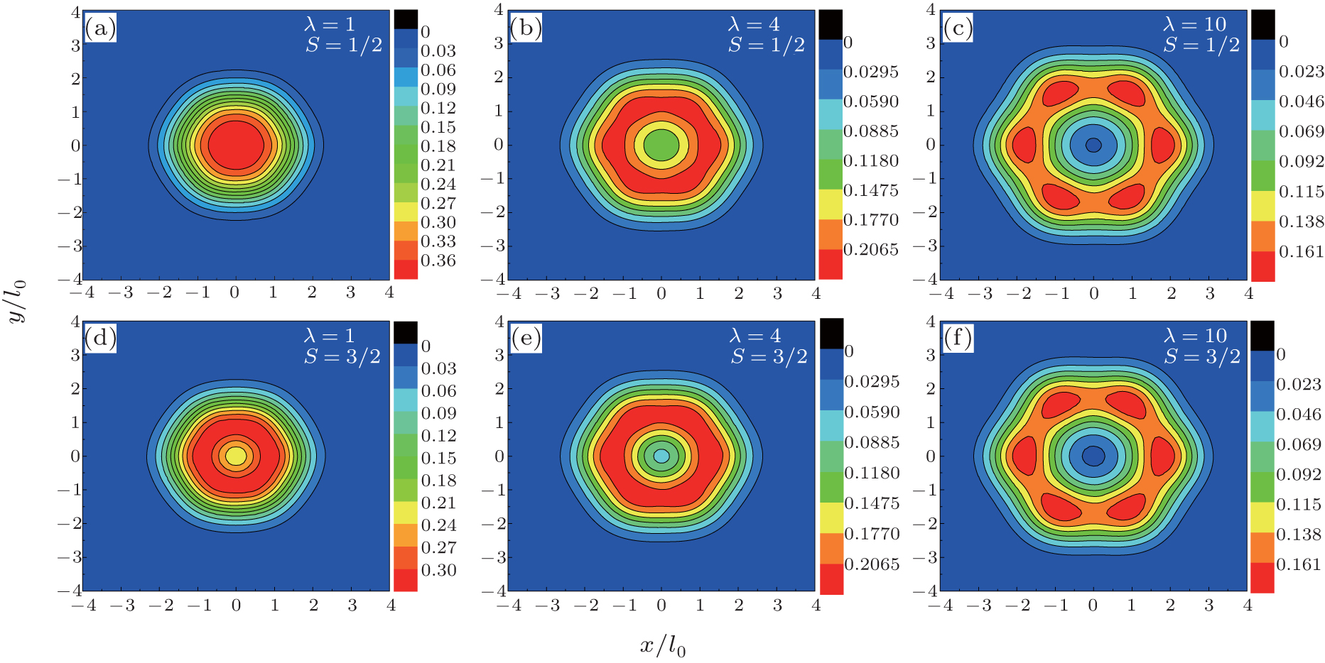	Fig. 2. Contour plots of total charge density distribution (in units of ) of three electrons in hexagonal quantum dot in the state S = 1/2 (first row) and S = 3/2 (second row) for (a), (d) λ = 1; (b), (e) λ = 4; (c), (f) λ = 10.

Fig. 3.

	Figure Option ViewDownloadNew Window
	Fig. 3. Contour plots of total charge density distribution (in units of ) of three electrons in square quantum dot in the state S = 1/2 (first row) and S = 3/2 (second row) for (a), (d) λ = 1; (b), (e) λ = 4; (c), (f) λ = 10.

Fig. 4.

	Figure Option ViewDownloadNew Window
	Fig. 4. Contour plots of total charge density distribution (in units of ) of three electrons in triangular quantum dot in the state S = 1/2 (first row) and S = 3/2 (second row) for (a), (d) λ = 1; (b), (e) λ = 4; (c), (f) λ = 10.

The charge density plots of triangular QD exhibit some distinct features from that of hexagonal and square QDs. Firstly, in strong interaction regime (λ = 10) for hexagonal and square QDs, although the localized density peaks are clear, they have some density connection. On the other hand, in the case of triangular QD the localization effects are more pronounced with respect to the other geometries since there are three independent and equal-sized peaks at the corners of the dot. This finding is inconsistent with the previous exact diagonalization results^[21] where the Wigner crystallization is observed in square and triangular QDs at high magnetic fields. Secondly, in hexagonal and square QDs, the S = 3/2 charge density at the center is smaller than that of S = 1/2 at λ = 1 and λ = 4 due to the exchange interaction. At λ = 10 the spindependency of the density distributions becomes very small. However, in the triangular QD, even at λ = 4, the charge densities belonging to two different spin states are almost the same.

The spin-independent charge density distribution, which denotes the formation of Wigner molecule, ^[11] is observed at a small λ value in comparison with the hexagonal and square QDs. Based on the information obtained from charge density distributions, it can be said that Wigner molecule formation is more apparent in the three-electron triangular QD. In Ref. [21] this behavior is interpreted by examining the relation between the quantum mechanical and classical charge densities. Classically, in a square and hexagonal confinement potential the three electrons form equivalent classical configurations (classical degeneracy). Whereas, in a triangular QD there is one configuration where three electrons occupy the corners of the dot. Therefore, as for three-electron triangular QD when the number of particles is compatible with the symmetry of the confining potential, i.e., in the absence of classical degeneracy, Wigner crystallization is seen more clearly.

In conclusion, we have investigated the ground-state spin and charge configurations of three-electron systems confined in polygonal QDs within the framework of the CI method. We have analyzed the dependence of the λ point, where the transition from S = 1/2 to S = 3/2 occurs, on the geometry of the confining potential. It has been found that decreasing the number of the sides of the dot suppresses the ground-state spin polarization. Observation of the charge densities of the polygonal QDs in different interaction regimes has shown that formation of Wigner molecule structure is more clear in the case of triangular shaped QD. Therefore, our results can be useful in better understanding the ground-state spin configurations and charge densities of many-electron systems confined in polygonal geometries.