


Application of Arnoldi method to boundary layer instability
[Zhang Yong-Ming†a), b)  , Luo Ji-Sheng
a) ]
, Luo Ji-Sheng|
|


†Corresponding author. E-mail: ymzh@tju.edu.cn
*Project supported by the National Natural Science Foundation of China (Grant Nos. 11202147, 11332007, 11172203, and 91216111) and the Specialized Research Fund for the Doctoral Program of Higher Education of China (Grant No. 20120032120007).
The Arnoldi method is applied to boundary layer instability, and a finite difference method is employed to avoid the limit of the finite element method. This modus operandi is verified by three comparison cases, i.e., comparison with linear stability theory (LST) for two-dimensional (2D) disturbance on one-dimensional (1D) basic flow, comparison with LST for three-dimensional (3D) disturbance on 1D basic flow, and comparison with Floquet theory for 3D disturbance on 2D basic flow. Then it is applied to secondary instability analysis on the streaky boundary layer under spanwise-localized free-stream turbulence (FST). Three unstable modes are found, i.e., an inner mode at a high-speed center streak, a sinuous type outer mode at a low-speed center streak, and a sinuous type outer mode at low-speed side streaks. All these modes are much more unstable than Tollmien–Schlichting (TS) waves, implying the dominant contribution of secondary instability in bypass transition. The modes at strong center streak are more unstable than those at weak side streaks, so the center streak is ‘dangerous’ in secondary instability.
Boundary layer transition is one of the fundamental problems of fluid mechanics, and it is greatly important for many engineering problems. For the flat plate boundary layer, there are two different kinds of transition mechanisms, i.e., natural transition and bypass transition.[1] In a quiet environment, natural transition occurs, whose typical process is as follows:[2] disturbances penetrate into the boundary layer via a receptivity mechanism and two-dimensional (2D) Tollmien– Schlichting (TS) waves are generated which can grow; when the amplitudes of the TS waves reach a high enough level, three-dimensional (3D) disturbances come into play via some mechanism, e.g., secondary instability and resonant triad interaction; then the growth of 3D disturbances leads to the turbulent boundary layer. On the other hand, at a high level of environmental disturbances, bypass transition occurs, whose typical process is as follows:[1] low-frequency disturbances penetrate into the boundary layer and streamwise streaks are generated; [3– 8] the growth of streaks is rapid so that secondary instability is triggered immediately, resulting in the growth of high-frequency disturbances; more and more turbulent spots occur somewhere in the boundary layer, and they merge to form a turbulent boundary layer. In the secondary instability stage of bypass transition, because the fundamental disturbances, i.e., low-frequency streaks, vary along both wall-normal and spanwise directions, an eigenvalue problem of 2D basic flow comes into being. For the bypass transition of a boundary layer under isotropic and axisymmetric FST, Zhang et al.[1] investigated the development of streaks and the secondary instability. For other typical cases, i.e., spanwise-localized FST, Zhang et al.[1] studied the streaks in the boundary layer by calculating nonlinear boundary-region equations, and found that there is a strong streak at the center and a weak one on each side. While the central one is high-speed, the other two are low-speed, and vice versa. However, secondary instability of the streaky boundary layer has not been investigated. Furthermore, for the boundary layer over complex geometry, such as the junction of an aircraft’ s nose and front wing, and the inlet of an aeroengine with a disturbance generator, in order to investigate its transition, the spanwise variation of basic flow should be taken into consideration from the beginning, implying that the fundamental instability of the boundary layer involves the eigenvalue problem of 2D basic flow. This kind of eigenvalue problem of 2D, even 3D, basic flow is named global linear instability.[9]
The parameters of TS waves in natural transition are obtained by solving the eigenvalue problem of Orr– Sommerfeld (OS) equations, whose basic flow varying along the wall-normal direction is 1D. For this problem, there have been mature methods, such as the Muller method.[2] However, it is hard to apply these methods to 2D basic flow due to the enormous computation cost. Floquet theory is used to investigate the inviscid problem of 2D basic flow successfully, [10, 11] and it is also useful in other fields.[12, 13] Although Floquet theory is convenient for the inviscid problem, it is quite complicated for a viscous problem and the computation cost is expensive.[14, 15] Vaughan and Zaki[15] employed viscous Floquet theory to streaky boundary layer instability, and found three kinds of unstable modes, i.e., inner mode, sinuous type outer mode, and varicose type outer mode. Phase speed of inner mode is low, while that of outer mode is high. The eigenfunction of the inner mode concentrates symmetrically at the bottom of the high-speed streak. The eigenfunction of the sinuous type outer mode concentrates antisymmetrically at two ‘ shoulders’ of the low-speed streak, while that of the varicose type outer mode concentrates symmetrically at the ‘ head’ and two ‘ shoulders’ of the low-speed streak.
As the development of computational mathematics, Arnoldi iteration has been used to boundary layer instability.[16– 18] The main idea is that the linearized disturbance equations are treated as a linear operator, and the eigenvalue problem of the operator is solved by iteration. By means of projection onto a small Krylov subspace, the eigenvalue problem of a large matrix is transformed to a small matrix, making the problem much easier to solve. Furthermore, many eigenmodes can be found by one run of Arnoldi iteration. In the conventional Arnoldi method, [16– 18] the finite element method is used to solve disturbance equations, so that it can be applied to complex geometry problems conveniently. However, for high-Reynolds-number problems, the convergence speed of the finite element method becomes slow, even unattainable. Furthermore, there are shock waves in high-speed compressible flow, especially in supersonic and hypersonic flows, which are hard for the finite element method to deal with. As a result, the conventional Arnoldi method is often applied to low-Reynolds-number incompressible problems. On the other hand, for the finite difference method there is no Reynolds-number limitation, although it can only be applied to regular geometry problems. Usually, in mechanism investigations, the geometry of the flow field is regular, so the finite difference method is effective for them. Furthermore, the finite difference method is effective for compressible, supersonic and hypersonic flows with shock waves. In common engineering problems, especially in aeronautics and aerospace, the Reynolds number is quite high usually, and there are shock waves in flow fields sometimes. Consequently, it is necessary to replace the finite element method in the conventional Arnoldi method by the finite difference method as done by Merle et al.[19] and in this paper. The method is applied to the instability of the boundary layer in this paper, while it is applied to the instability of the lid-driven cavity by Merle et al.[19] The performance of the Arnoldi method at a large Reynolds number is investigated, including accuracy and convergence. As the starting point, the incompressible problem is considered in this paper. In addition, in the conventional Arnoldi method, [17, 18] the eigenvalue package LAPACK[20] is used. In this paper, a more advanced package ARPACK[21] is used, whose interface is more convenient to edit.
The governing equations and numerical method of the Arnoldi method used in this paper are described in Section 2. The finite difference method is employed to solve linear stability equations, so that we can avoid the limit of the finite element method mentioned above. For the application of our Arnoldi method in investigation of the boundary layer instability, its effectiveness should be verified first. In Section 3, three comparative cases are examined in the sequence from easy to hard. Although the Arnoldi method in this paper is for 2D basic flow, its verification in 1D basic flow is still necessary as the starting point. The first case is for 2D disturbance on 1D basic flow (only depends on the wall-normal direction), and the results are compared with those of LST. The second case is for 3D disturbance in 1D basic flow, and the results are also compared with those of LST. The last case is for 3D disturbance in 2D basic flow, and the Reynolds number grows gradually so that the results can be compared with those of inviscid Floquet theory.[10] In Section 4, the Arnoldi method is applied to secondary instability analysis on the streaky boundary layer under spanwise-localized FST obtained by Zhang et al.[1] The conclusions are drawn from the present study in Section 5.
Starting from the full Navier– Stokes (NS) equations, the linearized disturbance equations are obtained.
The nondimensional incompressible NS equations in 3D Cartesian coordinates are
where x, y, and z represent streamwise, wall-normal and spanwise directions, respectively; u, v, and w represent instantaneous velocity components in three directions, respectively; p is the instantaneous pressure. The equations have been nondimensionalized by free-stream velocity U* and local boundary layer displacement thickness δ * , and the Reynolds number is Re = U* δ * /υ * , where υ * is the kinematic viscosity in the free-stream.
The instantaneous quantities are decomposed into the sum of basic flow and disturbance as follows:

where q = (u, v, w, p)T represents the vector of instantaneous quantities, U = (U, V, W, P)T the vector of basic flow, q′ = (u′ , v′ , w′ , p′ )T the vector of disturbance, and ε the amplitude of disturbance.
Substituting Eq. (2) into Eq. (1) and subtracting the equations corresponding to the basic flow, the disturbance equations are obtained. Then neglecting the nonlinear terms, the linearized disturbance equations are obtained as follows:
The periodic assumption is used in the streamwise direction as follows:

where q̂ = (û , v̂ , ŵ , p̂ )T, α is the streamwise wave number, c.c. represents complex conjugate. Substituting Eq. (4) into Eq. (3), the equations of q̂ are obtained as follows:

Equation (5) is the linear stability equations of 2D basic flow, and is the governing equation to be solved in this paper. A non-slip condition is imposed on the wall, and the perturbation at the top boundary is set to be zero as the far-field condition.
Equation (5) is a linear equation of q̂ . For a streamwise wave number α , equation (5) difines a linear evolution operator B(t, α ) which evolves disturbances forward in time, namely

Setting the time t to be a fixed value T, the operator becomes

where B(T, α ) is also a linear operator, for which there is an eigenvalue problem as follows:

where λ and q̇ (y, z) are the eigenvalue and eigenfunction of B(T, α ), respectively.
On the other hand, the evolution of q̂ from t = 0 to t = T can also be described by complex frequency ω as follows:

where ω = ω r + iω i, whose real and imaginary parts represent frequency and growth rate, respectively. Then an eigenmode can also be described as

In view of Eqs. (8) and (10), the relationship between eigenvalue λ and complex frequency ω is

and ω is used to represent the eigenvalue in the paper below.
The numerical method to solve Eq. (5) is presented below.
In the spanwise direction, q̂ is expressed as a Fourier series, namely
where β is the fundamental wave number in the spanwise direction. This implies that the uniform grid and periodic boundary condition are employed in this direction.
For the stable calculation of Eq. (5), 2D basic flow U(y, z) is decomposed into the sum of the one-dimensional part Ua(y) and two-dimensional part Ub (y, z) as follows:

where Ua is the spanwise mean value of U, namely
with Lz = 2π /β being the fundamental wave length; Ub is expressed as a Fourier series

Non-uniform grids with a denser distribution near the wall are employed in the wall-normal direction. For the application of a high order difference scheme, the equations are transformed into the computational coordinate, in which the grids are uniform, by the transformation η = η (y). The transformation in this paper is as follows:

where yl is the domain size and b is a constant given as

Here, constant kt is the rate of top space over bottom space.
The η derivatives are approximated by the fourth-order central difference schemes as follows:

For the points next to the top and bottom boundaries, they are replaced by the lower order ones.
For the time splitting, third-order difference scheme is employed, namely

For the first and second step, first- and second-order schemes are used, respectively.
The evolution of q̂ from t = 0 to t = T is obtained by solving Eq. (5). The eigenvalue problem of operator B(T, α ), i.e., the eigenmode including eigenvalue λ and eigenfunction q̇ (y, z), is calculated by Arnoldi iteration. This process is implemented by utilizing the package ARPACK.[21] The algorithm of Arnoldi iteration is illustrated briefly below, more details can be seen in Refs. [17] and [21].
Letting the operator B(T, α ) act on an arbitrary initial vector q̂ 0k times, which is of unit norm, i.e., ‖ q̂ 0‖ = 1, one obtains a Krylov sequence [q̂ 0, Bq̂ 0, B2q̂ 0, … , Bkq̂ 0] with k + 1 vectors, whose corresponding sequence of normalized vectors is
where aj are norms of the vectors, and q̂ j are normalized vectors, i.e., ‖ q̂ j‖ = 1. If the vector q̂ 0 is N-dimensional, Tk+ 1 is an N × (k + 1) matrix. with N being the product of the discretized point number of q̂ 0 on the y– z space and 4, i.e., the number of three velocity components and pressure, and is a large number usually. The action of B(T, α ) on discretized q̂ 0 can be represented by an N × N matrix M, which is so large that its eigenvalue problem is quite hard for a conventional method. k is the size number of the Krylov sequence, which is set by the user and can be a small one.
The action of the operator B(T, α ) on matrix Tk = [q̂ 0, q̂ 1, q̂ 2, … , q̂ k− 1] can be described as

where 
Tk and Tk+ 1 are expressed in terms of QR decompositions

where Qk = [q̃ 0, q̃ 1, q̃ 2, … , q̃ k− 1] is an N × k matrix with orthogonal columns, Rk is a k × k upper triangular, and similarly for Qk+ 1 and Rk+ 1. The k and (k + 1) matrices agree where they overlap, e.g. Qk and Qk+ 1 are the same except that Qk+ 1 contains one more column q̃ k.
Defining a (k + 1) × k matrix

equation (23) can be expressed as

Here, 


where 
Letting ϒ k = [υ 0, υ 1, υ 2, … , υ k− 1] be the k × k matrix whose columns are normalized eigenvectors of Hk, with corresponding eigenvalues (λ 0, λ 1, λ 2, … , λ k− 1), then diagonalizing Hk in Eq. (26) gives


where Λ k is the k × k diagonal eigenvalue matrix of Hk, and Ψ k is the N × k matrix of normalized approximate Ritz eigenvectors of B(T, α ), namely

The residual error of eigenmode 𝜓 j and λ j is exactly expressed by the last term in Eq. (28), namely
where the scalar 
In general, if q̂ 0 becomes N-dimensional after discretization, the action of operator B(T, α ) can be represented by an N × N matrix M, which is so large usually that it is quite hard to solve its eigenvalue problem directly. In Arnoldi iteration, B(T, α ) is projected onto a k-dimensional Krylov space. Because k is much smaller than N, it is much easier to solve the eigenvalue problem of the k × k matrix Hk, that is, one can utilize the QR method. From the eigenmode of Hk, both eigenmode of B(T, α ) and its residual error can be obtained, see Eqs. (29) and (30). If the residual error is small enough, the eigenmode is accurate and the iteration stops. If the residual error is large, the iteration is kept on and the sequence Tk+ 1 is renewed until the residual error becomes smaller than a pre-set threshold, which is taken to be on the order of 10− 16 in this paper.
In this section, the Arnoldi method is verified by three comparison cases. Then it is applied to global linear instability analysis on the streaky boundary layer under spanwise-localized FST.
For the first case, the basic flow is a Blasius boundary layer, and only 2D disturbance is taken into consideration. Because the assumption of parallel flow is employed, the basic flow is only dependent on y, resulting in the fact that the results of LST obtained by the Muller method are effective, which can be taken as a reference.[2] The wall-normal domain is yl = 14.5, which is about five times the boundary layer thickness. Grid number is Ny = 500, and the transformation ratio in Eq. (4) is kt = 100. In the spanwise direction, domain size is zl = 0.4, and grid number is Nz = 4.
Figure 1 shows the growth rate ω i and frequency ω r against streamwise wavenumber α of 2D disturbance at Re = 1000. The points at upper and lower branches of the neutral curve and at the maximal growth curve are indicated.
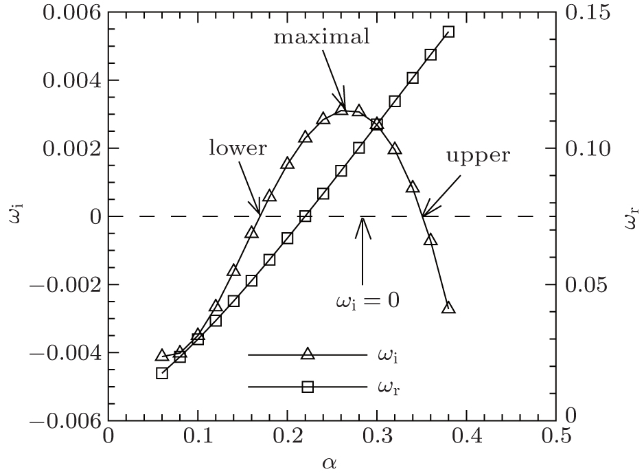 | Fig. 1. Growth rate ω i and frequency ω r against streamwise wavenumber α of 2D disturbance at Re = 1000 |
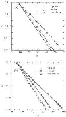
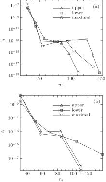
Figure 2 shows the plots of residual error ε r against iteration number ni at upper and lower branches of the neutral curve and at maximal growth curve at Re = 1000 and 4000. The residual errors decay monotonically during iterations. Because the finite difference method is employed, instead of the finite element method, there is no divergence problem.
 | Fig. 2. Plots of residual error ε r against iteration number ni at upper and lower branches of the neutral curve and at the maximal growth curve of 2D disturbance at Re = 1000 (a) and 4000 (b). Time period for each iteration is 20, and time step is 0.01. |
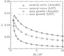
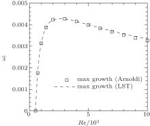
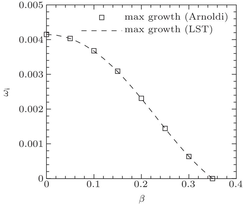
Figure 3 shows the neutral curve and maximal growth curve of 2D disturbances from the Arnoldi method and LST, and figure 4 shows the corresponding maximal growth rate. These figures show that the results of the Arnoldi method agree with those of LST, even at a large Reynolds number.
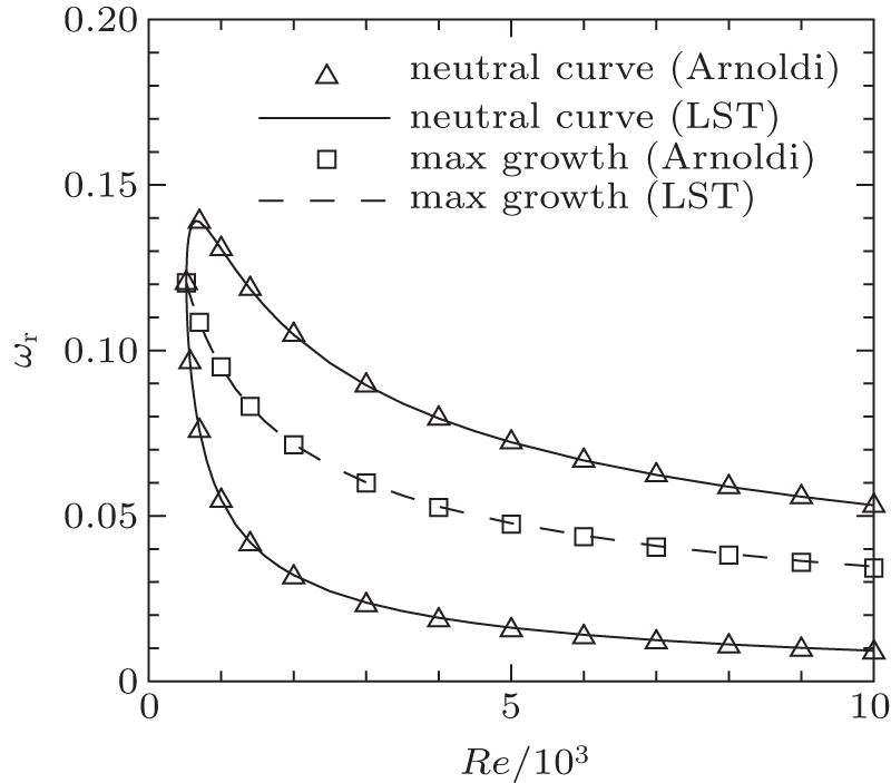 | Fig. 3. Neutral and maximal growth curves of 2D disturbance. |
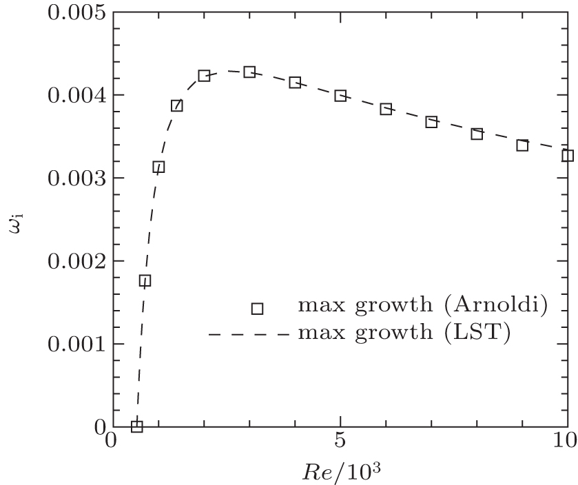 | Fig. 4. Maximal growth rate of 2D disturbance. |
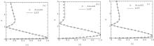
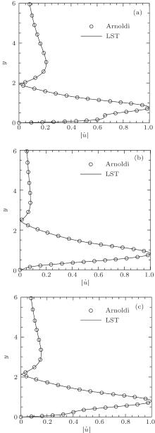
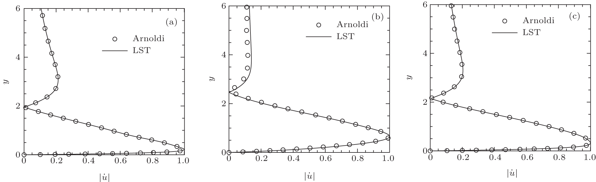
Figures 5 and 6 show the eigenfunction | u̇ | at Re = 1000 and 4000, respectively. The results at upper and lower branches of the neutral curve and at the maximal growth curve are taken into consideration, and all of them from Arnoldi agree quite well with those from LST.
 | Fig. 5. Eigenfunction | u̇ | of 2D disturbance at Re = 1000. (a) Upper branch of neutral curve, (b) lower branch of neutral curve, and (c) maximal growth curve. |
 | Fig. 6. Eigenfunction | u̇ | of 2D disturbance at Re = 4000. (a) Upper branch of neutral curve, (b) lower branch of neutral curve, and (c) maximal growth curve. |
The second case is also for the Blasius boundary layer, but 3D disturbance is considered. The LST results of Zhou and Zhao[2] are still taken as a reference. The domain size and grid in the wall-normal direction are the same as in the first case. In the spanwise direction, domain size is set to be zl = 2π /β , grid number is Nz = 8.
Figure 7 shows the growth rate ω i and frequency ω r against streamwise wavenumber α of 3D disturbances at β = 0.12 and Re = 1000. The points at the upper and lower branches of neutral curve and at the maximal growth curve are indicated.
 | Fig. 7. Growth rate ω i and frequency ω r against streamwise wavenumber α of 3D disturbance at β = 0.12 and Re = 1000. |
Figure 8(a) shows the plots of residual error ε r against iteration number ni at upper and lower branches of the neutral curve and at the maximal growth curve of 3D disturbance at Re = 1000. Unlike the first case, residual errors rise slightly at levels from 10− 13 to 10− 14. After that, they decay until convergence. Figure 8(b) shows the results at Re = 4000. The residual errors decay until convergence monotonically, and there is no divergence problem.
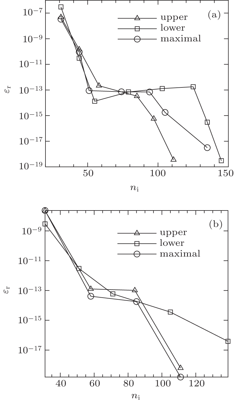 | Fig. 8. Plots of residual error ε r against iteration number ni at upper and lower branches of the neutral curve and at the maximal growth curve of 3D disturbance at Re = 1000 and 4000. (a) Re = 1000 and β = 0.12. Time period for each iteration is 20, and time step is 0.01. (b) Re = 4000 and β = 0.20. Time period for each iteration is 34, and time step is 0.017. |
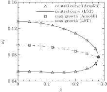
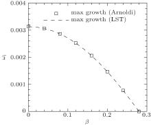
Figure 9 shows the neutral curve and maximal growth curve of 3D disturbance at Re = 1000, and figure 10 shows the corresponding maximal growth rate. Only the part of β ≥ 0 is shown, because the part of β < 0 is exactly symmetric with respect to it. These Figures show that the results of the Arnoldi method agree with those of LST quite well.
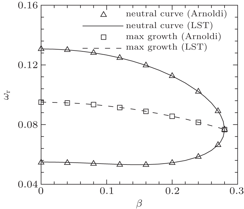 | Fig. 9. Neutral and maximal growth curves of 3D disturbance at Re = 1000. |
 | Fig. 10. Maximal growth rate of 3D disturbance at Re = 1000. |
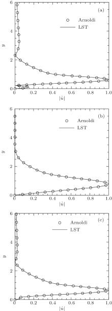
Figure 11 shows the eigenfunction | u̇ | at β = 0.12 and Re = 1000. The results at upper and lower branches of the neutral curve and at the maximal growth curve are taken into consideration, and all of them from Arnoldi agree with quite well with those from LST.
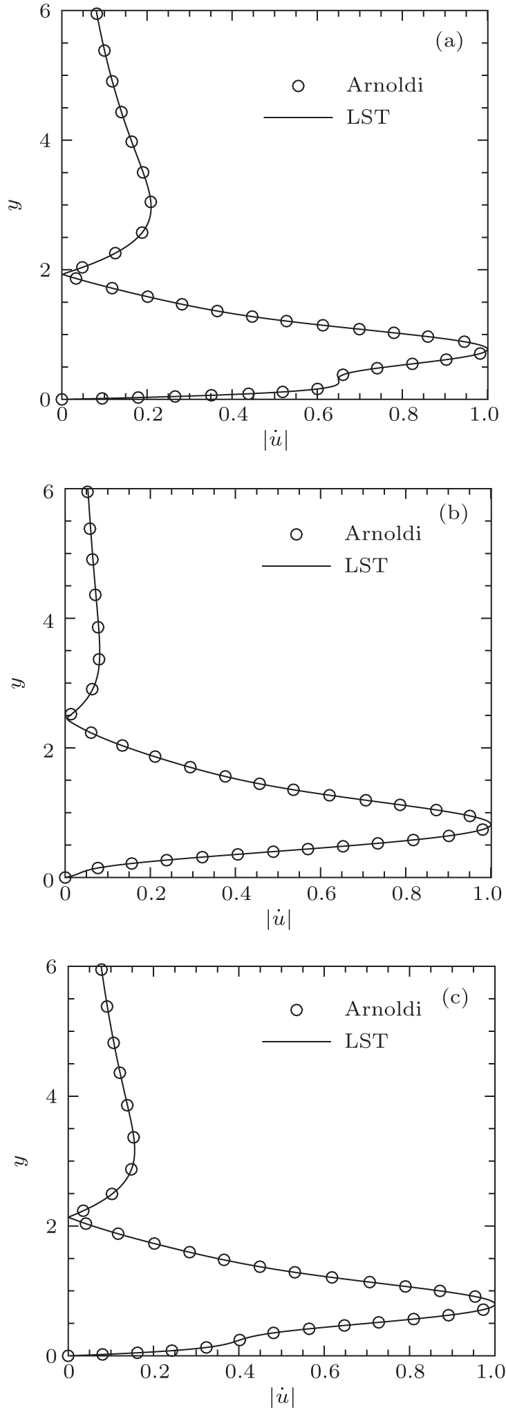 | Fig. 11. Eigenfunction | u̇ | of 3D disturbance at β = 0.12, Re = 1000. (a) | u̇ | at the upper branch of the neutral curve; (b) | u̇ | at the lower branch of the neutral curve; (c) | u̇ | at the maximal growth curve. |
Figures 12– 14 show the results of 3D disturbance at a larger Reynolds number Re = 4000. The situation is similar to that at Re = 1000.
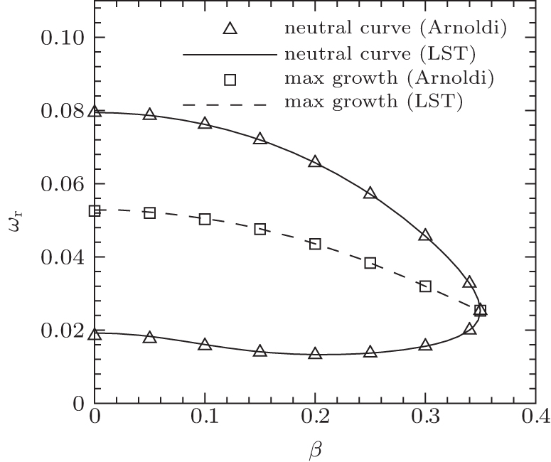 | Fig. 12. Neutral and maximal growth curves of 3D disturbance at Re = 4000. |
 | Fig. 13. Maximal growth rate of 3D disturbance at Re = 4000. |
 | Fig. 14. Eigenfunctions | u̇ | of 3D disturbance at β = 0.20, Re = 4000. (a) | u̇ | at the upper branch of the neutral curve; (b) | u̇ | at the lower branch of the neutral curve; (c) | u̇ | at the maximal growth curve. |
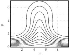
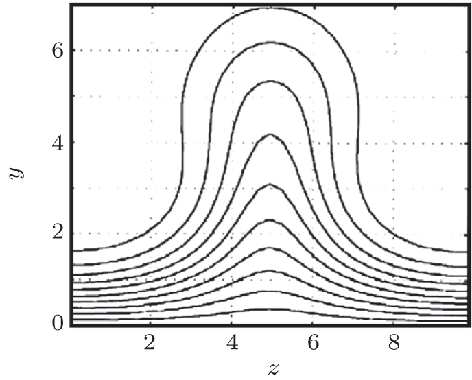
The third case is for 2D basic flow. The streaky boundary layer in Ref. [10] (Fig. 6(b), also see Fig. 15 in this paper) is taken into consideration, which is dependent on y and z. The streak is due to the low-frequency and long-wave-length disturbance, [4– 9] while the secondary instability is for high-frequency and short-wave-length disturbance. As a result, the parallel assumption is still available.
In Ref. [10], although the streaky basic flow is vicious with Reynolds number Re = 468, only the instability analysis result from the inviscid Floquet theory is given, which is taken as reference. The Floquet theory is for the inviscid flow, implying that the Reynolds number is Re = + ∞ . However, the Arnoldi method is for the viscous flow, implying that the Reynolds number must be limited. For comparison with the result of Floquet theory, one can increase the Reynolds number in the Arnoldi method gradually.
The streamwise wave number is α = 0.28 in this case.
The wall-normal domain is yl = 86. Grid number is Ny = 200, and the transformation ratio in Eq. (4) is kt = 300. In the spanwise direction, domain is zl = 9.875, and grid number is Nz = 64.
Tables 1 and 2 show frequency ω r and growth rate ω i, respectively. At a low Reynolds number, i.e., Re = 45, the results from the Arnoldi method are apparently different from those from the inviscid Floquet theory because of the viscous effects. As the Reynolds number increases, the results of the Arnoldi method change towards the inviscid values because the viscous effect becomes weak.
| Table 1. Arnoldi and Floquet[10]: frequency ω r. |
| Table 2. Arnoldi and Floquet[10]: growth rate ω i. |
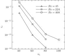
Figure 16 shows the plots of residual error ε r against iteration number ni at Re = 45, 224, and 468. The residual errors decay monotonically during iterations. As the Reynolds number increases, there is no divergence problem.
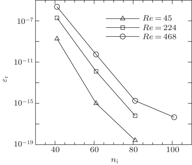 | Fig. 16. Plots of residual error ε r against iteration number ni at Re = 45, 224, and 468. Time period for each iteration is 11.11, and time step is 0.01111. |
Figure 17 shows the eigenfunction | u̇ | from the Arnoldi method at Re = 468 and that from the Floquet theory (Fig. 12(a) in Ref. [10]). Furthermore, the critical layer is also indicated in the figure, where the streamwise velocity of basic flow U equals the phase speed of disturbance Cr = ω r/α . The agreement between the results from the two methods is quite good.
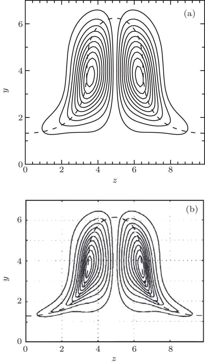 | Fig. 17. (a) Arnoldi (Re = 468) and (b) Floquet (Fig. 12(a) in Ref. [10]): eigenfunction | u̇ | (solid line: contours of eigenfunction | u̇ | ; dashed line: critical layer.) |
The studies of the above three cases show that the Arnoldi method works in the instability analysis of the boundary layer. It is still effective at a large Reynolds number because the finite difference is employed to solve disturbance equations. As a result, although the Arnoldi method is for incompressible flow in this paper, it is promising to extend it to compressible flow, especially super and hypersonic flows.
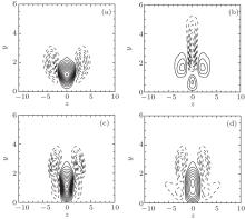
The verified method is applied to the secondary instability of the streaky boundary layer under the spanwise-localized free-stream turbulence. Zhang et al.[1] investigated the streaks under FST with different levels, and compared their numerical results with experimental data of Westin et al.[22] at x* = 160 mm, Re = 446. In the present paper, the secondary instability is studied for the free-stream turbulence level of ε l = 0.03. Because the streaks are of low-frequency, their time period is quite long. The streamwise size of the streaks is long as well. The dependences of the streaky boundary layer on x and t can be treated as being parametric when short wavelength (on the order of boundary layer thickness) and relevant high-frequency instability are considered as noted by Ricco et al.[11] At fixed x and t, the streaky basic flow depends on y and z only. In the case of the long time period, the following four time phases

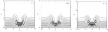
are taken, because the amplitude of the streamwise perturbation velocity up is relatively high at these instants as shown in Fig. 18. The central streak is low-speed at ϕ = 37π /128, and is high-speed at the other three ones.
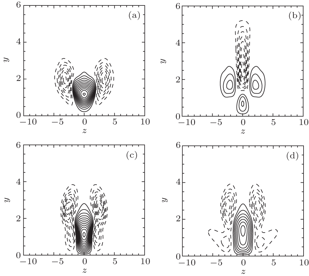 | Fig. 18. Streamwise perturbation velocity up at x* = 160 mm at time phases ϕ = 15 π /128 (a), 37π /128 (b), 81π /128 (c), and 121π /128 (d) under localized FST with level ε l = 0.03 (solid contour lines: positive values, and dashed contour lines: negative values. Contour spacing: 0.02). |
The wall-normal domain is yl = 24.2. Grid number is Ny = 200, and the transformation ratio in Eq. (4) is kt = 100. In the spanwise direction, domain is zl = 20.3, and grid number is Nz = 256.
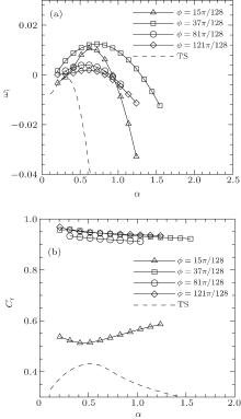
Figure 19(a) shows the plots of the growth rate ω i against streamwise wavenumber α , and the result of 2D TS waves for the Blasius flow is shown as well. Unstable disturbances are found at all four time phases, and their growth rates are much higher than that of the most unstable TS wave, implying that the contribution of secondary instability to bypass transition is much stronger than that of TS waves. The high growth rate can also explain why a bypass transition happens much earlier than a natural transition. It is interesting that the growth rate is always sensitive to steamwise wavenumber α ≈ 0.7 at different instants. This reminds us to pay attention to the ‘ dangerous’ wavenumber in the following investigation. Figure 19(b) shows the phase speed Cr. It is between 0.5 and 0.6 at ϕ = 37π /128, indicating these unstable modes are inner modes.[15] It is higher than 0.9 at other instants, indicating these modes are the outer mode.[15]
 | Fig. 19. Curves of growth rate ω i (a) and phase speed Cr (b) against streamwise wavenumber α at different time phases. |
Figure 20 shows the plots of residual error ε r against iteration number ni at the ‘ dangerous’ wavenumber α = 0.72 at four time phases. The residual errors decay monotonically during iterations, but the convergence speeds are different. At ϕ = 15π /128, the convergence speed is much quicker than the other cases. At ϕ = 121π /128, it is the slowest one in the four cases.
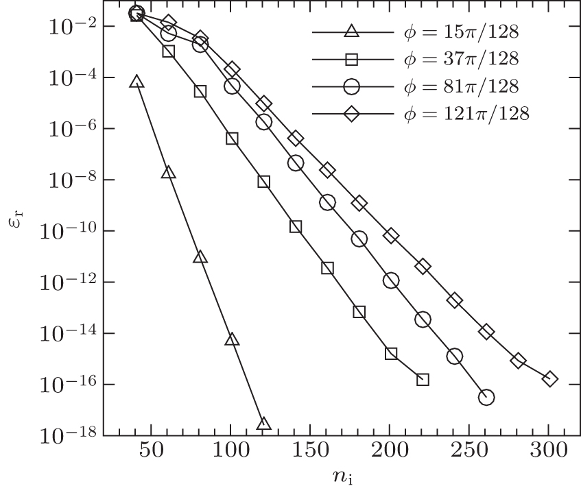 | Fig. 20. Plots of residual error ε r against iteration number ni at α = 0.72 and different time phases. Time period for each iteration is 2.91, and time step is 0.00485. |
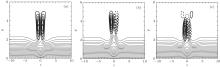
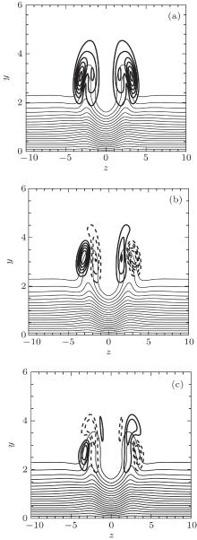
Figures 21– 24 show eigenfunction distributions of the unstable mode at α = 0.72 at four instants, respectively, including modulus| u̇ | , real part u̇ r, and imaginary part u̇ i. The streamwise velocity of streaky basic flow is shown as well. At ϕ = 15π /128, eigenfunction appears at the bottom of the high-speed center streak, and both real and imaginary parts are symmetric in the spanwise direction. The eigenfunction distribution and low phase speed (see Fig. 19(b)) of the mode indicate that it is the inner mode.[15] At ϕ = 37π /128, an eigenfunction appears at two ‘ shoulders’ of the low-speed center streak, and both real and imaginary parts are antisymmetric in the spanwise direction. The eigenfunction distribution and high phase speed (see Fig. 19(b)) of the mode indicate that they are in the sinuous type outer mode.[15] At ϕ = 81π /128 and 121π /128, an eigenfunction appears at two ‘ shoulders’ of each low-speed side streak, and both real and imaginary parts are antisymmetric in the spanwise direction. The eigenfunction distribution and high phase speed (see Fig. 19(b)) of the modes indicate that they are in the sinuous type outer mode.[15] Figure 19(a) shows that the growth rates at ϕ = 15π /128 and 37π /128 are much higher than those at ϕ = 81π /128 and 121π /128, implying that the unstable modes at the central streak are more unstable than those at side streaks.
 | Fig. 21. Contours of modulus (a), real part (b), and imaginary part (c) of eigenfunction u̇ at ϕ = 15π /128. |
 | Fig. 22. Contours of modulus (a), real part (b), and imaginary part (c) of eigenfunction u̇ at ϕ = 37π /128. |
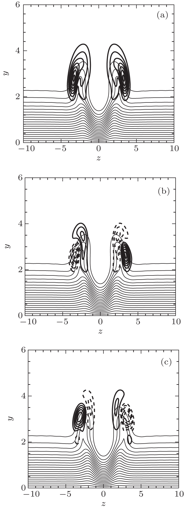 | Fig. 23. Contours of modulus (a), real part (b), and imaginary part (c) of eigenfunction u̇ at ϕ = 81π /128. |
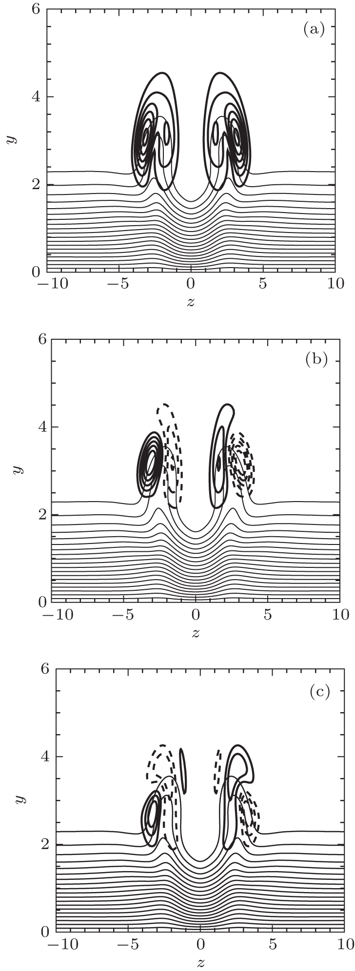 | Fig. 24. Contours of modulus (a), real part (b), and imaginary part (c) of eigenfunction u̇ at ϕ = 121π /128. |
Solid thick lines: positive contours of eigenfunction; dashed thick lines: negative contours of eigenfunction; thin lines: contours of streamwise velocity of the streaky boundary layer with contour spacing 0.05.
The Arnoldi method is used to investigate the boundary layer instability. During the iteration, the finite difference method is employed to solve disturbance equations, so that the limits of the finite element method at a large Reynolds number and for shock waves are avoided. The method is verified by three calculation cases, i.e., 2D disturbance on 1D basic flow, 3D disturbance on 1D basic flow, and 3D disturbance on 2D basic flow. It should be noted that the method still works at a large Reynolds number.
The verified method is applied to secondary instability of the streaky boundary layer under spanwise-localized FST, and three kinds of unstable modes are found, i.e. an inner mode at the high-speed center streak, a sinuous type outer mode at the low-speed center streak, and a sinuous type outer mode at low-speed side streaks. The growth rates of these modes are much higher than that of TS waves, so the contribution of secondary instability is dominant in bypass transition. This is also the reason for the early occurrence of bypass transition. The modes at the strong center streak are much more unstable than those at weak side streaks, implying that they play the key roles in secondary instability, and that they have the potential to induce turbulent spot and lead to transition consequently.
The authors are grateful to Prof. Brandt Luca of KTH Royal institute of Technology for providing the data in Ref. [
| 1 |
|
| 2 |
|
| 3 |
|
| 4 |
|
| 5 |
|
| 6 |
|
| 7 |
|
| 8 |
|
| 9 |
|
| 10 |
|
| 11 |
|
| 12 |
|
| 13 |
|
| 14 |
|
| 15 |
|
| 16 |
|
| 17 |
|
| 18 |
|
| 19 |
|
| 20 |
|
| 21 |
|
| 22 |
|